Storage Myths: Dedupe for Databases

Storage for DBAs: Data deduplication – or “dedupe” – is a technology which falls under the umbrella of data reduction, i.e. reducing the amount of capacity required to store data. In very simple terms it involves looking for repeating patterns and replacing them with a marker: as long as the marker requires less space than the pattern it replaces, you have achieved a reduction in capacity. Deduplication can happen anywhere: on storage, in memory, over networks, even in database design – for example, the standard database star or snowflake schema. However, in this article we’re going to stick to talking about dedupe on storage, because this is where I believe there is a myth that needs debunking: databases are not a great use case for dedupe.

Deduplication Basics: Inline or Post-Process

If you are using data deduplication either through a storage platform or via software on the host layer, you have two basic choices: you can deduplicate it at the time that it is written (known as inline dedupe) or allow it to arrive and then dedupe it at your leisure in some transparent manner (known as post-process dedupe). Inline dedupe affects the time taken to complete every write, directly affecting I/O performance. The benefit of post-process dedupe therefore appears to be that it does not affect performance – but think again: post-process dedupe first requires data to be written to storage, then read back out into the dedupe algorithm, before being written to storage again in its deduped format – thus magnifying the amount of I/O traffic and indirectly affecting I/O performance. In addition, post-process dedupe requires more available capacity to provide room for staging the inbound data prior to dedupe.

Deduplication Basics: (Block) Size Matters

In most storage systems dedupe takes place at a defined block size, whereby each block is hashed to produce a unique key before being compared with a master lookup table containing all known hash keys. If the newly-generated key already exists in the lookup table, the block is a duplicate and does not need to be stored again. The block size is therefore pretty important, because the smaller the granularity, the higher the chances of finding a duplicate:

In the picture you can see that the pattern “1234”repeats twice over a total of 16 digits. With an 8-digit block size (the lower line) this repeat is not picked up, since the second half of the 8-digit pattern does not repeat. However, by reducing the block size to 4 digits (the upper line) we can now get a match on our unique key, meaning that the “1234” pattern only needs to be stored once.

This sounds like great news, let’s just choose a really small block size, right? But no, nothing comes without a price – and in this case the price comes in the size of the hashing lookup table. This table, which contains one key for every unique block, must range in size from containing just one entry (the “ideal” scenario where all data is duplicated) to having one entry for each block (the worst case scenario where every block is unique). By making the block size smaller, we are inversely increasing the maximum size of the hashing table: half the block size means double the potential number of hash entries.

Hash Abuse

Why do we care about having more hash entries? There are a few reasons. First there is the additional storage overhead: if your data is relatively free of duplication (or the block size does not allow duplicates to be detected) then not only will you fail to reclaim any space but you may end up using extra space to store all of the unique keys associated with each block. This is clearly not a great outcome when using a technology designed to reduce the footprint of your data. Secondly, the more hash entries you have, the more entries you need to scan through when comparing freshly-hashed blocks during writes or locating existing blocks during reads. In other words, the more of a performance overhead you will suffer in order to read your data and (in the case of inline dedupe) write it.

If this is sounding familiar to you, it’s because the hash data is effectively a database in which storage metadata is stored and retrieved. Just like any database the performance will be dictated by the volume of data as well as the compute resource used to manipulate it, which is why many vendors choose to store this metadata in DRAM. Keeping the data in memory brings certain performance benefits, but with the price of volatility: changes in memory will be lost if the power is interrupted, so regular checkpoints are required to persistent storage. Even then, battery backup is often required, because the loss of even one hash key means data corruption. If you are going to replace your data with markers from a lookup table, you absolutely cannot afford to lose that lookup table, or there will be no coming back.

Database Deduplication – Don’t Be Duped

Now that we know what dedupe is all about, let’s attempt to apply it to databases and see what happens. You may be considering the use of dedupe technology with a database system, or you may simply be considering the use of one of a number of recent storage products that have inline dedupe in place as an “always on” option, i.e. you cannot turn it off regardless of whether it helps or hinders. The vendor may make all sorts of claims about the possibilities of dedupe, but how much benefit will you actually see?

Let’s consider the different components of a database environment in the context of duplication:

Oracle datafiles contain data blocks which have block headers at the start of the block. These contain numbers which are unique for each datafile, making deduplication impossible at the database block size. In addition, the end of each block contains a tailcheck section which features a number generated using data such as the SCN, so even if the block were divided into two the second half would offer limited opportunity for dedupe while the first half would offer none.
Even if you were able to break down Oracle blocks into small enough chunks to make dedupe realistic, any duplication of data is really a massive warning about your database design: normalise your data! Also, consider features like index key compression which are part of the Enterprise Edition license.
Most Oracle installations have multiplexed copies of important files like online redo logs and controlfiles. These files are so important that Oracle synchronously maintains multiple copies in order to ensure against data loss. If your storage system is deduplicating these copies, this is a bad thing – particularly if it’s an always on feature that gives you no option.
While unallocated space (e.g. in an ASM diskgroup) might appear to offer the potential for dedupe, this is actually a problem which you should solve using another storage technology: thin provisioning.
You may have copies of datafiles residing on the same storage as production, which therefore allow large-scale deduplication to take place; perhaps they are used as backups or test/development environments. However, in the latter case, test/dev environments are a use case for space-efficient snapshots rather than dedupe. And if you are keeping your backups on the same storage system as your production data, well… good luck to you. There is nothing more for you here.
Maybe we aren’t talking about production data at all. You have a large storage array which contains multiple copies of your database for use with test/dev environments – and thus large portions of the data are duplicated. Bingo! The perfect use case for storage dedupe, right? Wrong. Database-level problems require database-level solutions, not storage-level workarounds. Get yourself some licenses for Delphix and you won’t look back.

To conclude, while dedupe is great in use cases like VDI, it offers very limited benefit in database environments while potentially making performance worse. That in itself is worrying, but what I really see as a problem is the way that certain storage vendors appear to be selling their capacity based on assumed levels of dedupe, i.e. “Sure we are only giving you X terabytes of storage for Y price, but actually you’ll get 10:1 dedupe which means the price is really ten times lower!”

Sizing should be based on facts, not assumptions. Just like in the real world, nothings comes for free in I.T. – and we’ve all learnt that the hard way at some point. Don’t be duped.

Understanding Disk: Over-Provisioning

Storage for DBAs: In a recent news article in the UK, supermarket giant Tesco said it threw away almost 30,000 tonnes of food in the first half of 2013. That’s about 33,000 tons for those of you who can’t cope with the metric system. The story caused a lot of debate about the way in which we ignore the issue of wasted food – with Tesco being both criticised for the wastage and praised for publishing the figures. But waste isn’t a problem confined to just the food industry. The chances are it’s happening on your data centre too.

Stranded Capacity

As a simple example, let’s take a theoretical database which requires just under 6TB of storage capacity. To avoid complicating things we are going to ignore concepts such as striping, mirroring, caching and RAID for a moment and just pretend you want to stick a load of disks in a server. How many super-fast 15k RPM disk drives do you need if each one is 600GB? You need about ten, more or less, right? But here’s the thing: the database creates a lot of random I/O so it has a peak requirement for around 20,000 physical IOPS (I/O operations per second). Those 600GB drives can only service 200 IOPS each. So now you need 100 disks to be able to cope with the workload. 100 multiplied by 600GB is of course 60TB, so you will end up deploying sixty terabytes of capacity in order to service a database of six terabytes in size. Welcome to over-provisioning.

Now here’s the real kicker. That remaining 54TB of capacity? You can’t use it. At least, you can’t use it if you want to be able to guarantee the 20,000 IOPS requirement we started out with. Any additional workload you attempt to deploy using the spare capacity will be issuing I/Os against it, resulting in more IOPS. If you were feeling lucky, you could take a gamble on trying to avoid any new workloads being present during peak requirement of the original database, but gambling is not something most people like to do in production environments. In other words, your spare capacity is stranded. Of your total disk capacity deployed, you can only ever use 10% of it.

Of course, disk arrays in the real world tend to use concepts such as wide-striping (spreading chunks of data across as many disks as possible to take advantage of all available performance) and caching (staging frequently accessed blocks in faster DRAM) but the underlying principle remains.

Short Stroking

If that previous example makes you cringe at the level of waste, prepare yourself for even worse. In my previous article I talked about the mechanical latency associated with disk, which consists of seek time (the disk head moving across the platter) and rotational latency (the rotation of the platter to the correct sector). If latency is critical (which it always, always is) then one method of reducing the latency experienced on a disk system is to limit the movement of the head, thus reducing the seek time. This is known as short stroking. If we only use the outer sectors of the platter (such as those coloured green in the diagram here), the head is guaranteed to always be closer to the next sector we require – and note that the outer sectors are preferable because they have a higher transfer rate than the inner sectors (to understand why, see the section on zones in this post). Of course this has a direct consequence in that a large portion of the disk is now unused, sometimes up to 90%. In the case of a 600GB disk short stroking may now result in only 60GB of capacity, which means ten times as many disks are necessary to provide the same capacity as a disk which is not short stroked.

Two Types of Capacity

When people talk about disk capacity then tend to be thinking of the storage capacity, i.e. the number of bytes of data that can be stored. However, while every storage device must have a storage capacity, it will also have a performance capacity – a limit to the amount of performance it can deliver, measured in I/Os per second and/or some derivative of bytes per second. And the thing about capacities is that bad things tend to happen when you try to exceed them.

In simplistic terms, performance and storage capacity are linked, with the ratio between them being specific to each type of storage. With disk drives, the performance capacity usually becomes the blocker before the storage capacity, particularly if the I/O is random (which means high numbers of IOPS). This means any overall solution you design must exceed the required storage capacity in order to deliver on performance. In the case of flash memory, the opposite is usually true: by supplying the required storage capacity there will be a surplus of performance capacity. Provide enough space and you shouldn’t need to worry about things like IOPS and bandwidth. (Although I’m not suggesting you should forego due diligence and just hope everything works out ok…)

Waste Watching

I opened with a reference to the story about food wastage – was it fair to compare this to wasted disk capacity in the data centre? One is a real world problem and the other a hypothetical idea taking place somewhere in cyberspace, right? Well maybe not. Think of all those additional disks that are required to provide the performance capacity you need, resulting in excess storage capacity which is either stranded or (in the case of short stroking) not even addressable. All those spindles require power to keep them spinning – power that mostly comes from power stations burning fossil fuels. The heat that they produce means additional cooling is required, adding to the power draw. And the additional data centre floor space means more real estate, all of which costs money and consumes resources. It’s all waste.

And that’s just the stuff you can measure. What about the end users that have to wait longer for their data because of the higher latency of disk? Those users may be expensive resources in their own right, but they are also probably using computers or smart devices which consume power, accessing your database over a network that consumes more power, via application servers that consume yet more power… all wasting time waiting for their results.

Wasted time, waster money, wasted resources. The end result of over-provisioning is not something you should under-estimate…

Understanding Disk: Mechanical Limitations

Storage for DBAs: The year 2000. Remember that? The IT industry had just spent years making money off the back of the millenium bug (which turned out not to exist). The world had spent even more money than usual on fireworks, parties and alcohol. England failed to win an international football tournament again (some things never change). It was all quite a long time ago.

It was also an important year in the world of disk drive manufacturing, because in February 2000 Seagate released the Cheatah X15 – the world’s first disk drive spinning at 15,000 rotations per minute (RPM). At the time this was quite a milestone, because it came only four years after the first 10k RPM drive (also a Seagate Cheetah) had been released. The 50% jump from 10k to 15k made it look like disks were on a path of continual acceleration… and yet now, as I write this article in 2013, 15k remains the fastest disk drive available. What happened?

Disks haven’t completely stagnated. They continue to get both larger and smaller: larger in terms of capacity, smaller in terms of form factor. But they just aren’t getting any faster…

You don’t need to take my word for this. This technology paper (from none other than Seagate themselves) contains the following table on page 2:

Document TP-525 - Seagate Global Product Marketing (May 2004) — Document TP-525 – Seagate Global Product Marketing (May 2004)

Published in 2004, this document shows that between 1987 and 2004 the performance of CPU increased by a factor of two million, while disk drive performance increased by a factor of just eleven. And that was over a decade ago, so CPU has improved many times more since then. Yet the 15k RPM drive remains the upper limit of engineering for rotating media – and this is unlikely to change, for reasons I will explain in a minute. But first, a more basic question: why do we care?

Seek Time and Rotational Latency

As we discussed previously, a hard drive contains one or more rotating aluminium disks (known as “platters“) which are coated in a ferromagnetic material used to magnetically store bits (i.e. zeros and ones). In the case of a 15k RPM drive it is the platter that rotates 15,000 times per minute, or 250 times per second. Data is read from and written to the platter by a read/write head mounted on top of an actuator arm which moves to seek out the desired track. Once the head is above this track, the platter must rotate to the start of the required sector – and only at this point does the I/O begin.

Both of those mechanical actions take time – and therefore introduce delays into the process of performing I/O. The time taken to move the head to the correct track is known as the seek time, while the time taken to rotate the platter is called the rotational latency. Since the platter does not stop spinning during normal operation, it is not possible to perform both actions concurrently – if the platter spins to the correct sector before the head is above the right track, it must continue to spin through another revolution.

Now obviously, both of these wait times are highly dependant on where the head and platter were prior to the I/O call. In the best case, the head does not need to move at all and the platter is already at the correct sector, requiring zero wait time. But in the worst case, the head has to travel from one edge to the other and then the platter needs to rotate 359 degrees to start the read or write. Each I/O is like a throw of the dice, which is why when we discuss latency we have to talk in averages.

Modern enterprise disk drives such as this Seagate Cheetah 15K.7 SAS drive have average seek times of around 3.5ms to 4ms – although in a later article I will talk about how this can be reduced. Rotational latency is a factor of the speed at which the platter rotates – hence the interest in making disks that spin at 15k RPM or faster. At 15,000 revolutions per minute, each revolution takes 4ms, meaning the set of all possible latencies ranges from 0ms to 4ms. Once you consider it like that, it’s pretty obvious that the average rotational latency of a 15k RPM drive is 2ms. You can use the same method to calculate that a 10k RPM drive has an average of 3ms and so on.

Why Not Spin Faster?

A surprisingly-common misconception about disk drives is that the head touches the platter, in the same way as a vinyl record player has a needle/stylus that touches the record (for any younger readers: this is how we used to live). But in a disk drive, the head “flies” above the platter at a distance of a few nanometers, using airflow to keep itself in place (similar to the concept of a fluid bearing).

There are three main problems with making disks that revolve faster than 15k, the first of which is energy: the power consumption required to create all of that additional kinetic energy, as well as the associated heat it creates. At a time when energy costs are constantly increasing, customers do not want to pay even more money for devices that require more power and more cooling to run.

A more fundamental problem is related to aerodynamics, in that by rotating the platter faster the platter’s outer edge starts to travel at very high speed causing it to interact negatively with the surrounding air (a phenomenon known scientifically as flutter). For a 3.5 inch platter, the outer edge is travelling at approximately 150 miles per hour. It isn’t possible to remove the air, because this would result in the head touching the platter – causing devastation. One potential solution is to reduce the diameter of the platter, e.g. 2.5 inches or less (thereby reducing the speed of the edge) but this results in reduced disk capacity. Some manufacturers are replacing the air with helium in an attempt to reduce flutter and buffeting, but helium is both expensive and scarce, while the manufacturing process is undoubtedly more complex.

But the biggest – and potentially insurmountable – problem is the cost. Technical challenges can (mostly) be overcome, but customers will not pay for products that do not make economic sense. Disks are built and sold in large volumes, so any new manufacturing process requires a heavy investment – essentially a gamble taken by the manufacturer on whether customers will buy the new product or not. It’s unlikely we’ll see anything faster than 15k RPM manufactured in volume, because there simply isn’t the demand. Not when there are so many cheaper workarounds…

Spin Doctors

As the old saying goes, necessity is the mother of invention. Give people enough time to work around a problem and you will get all sorts of interesting tricks, hacks and dodges. And in the case of disk performance, we’ve been suffering from the limitations of mechanical latency for decades. The next articles in this series will look at some of the more common strategies employed to avoid, or limit, the impact of mechanical latency to disk performance: over-provisioning, short-stroking, caching, tiering… But rest assured of one thing: they are all just attempts at hiding the problem. Ultimately, the only way to remove the pain of mechanical latency is to remove the mechanics. By moving to semiconductor-based storage, all of the delays introduced by moving heads and spinning platters simply disappear… in a flash.

Understanding Disk: Superpowers

Storage for DBAs: It’s a familiar worn-out story. A downtrodden and oppressed population are rescued from their plight by a mysterious superhero. Over time they come to rely on this new superbeing – taking him for granted even, complaining when he isn’t immediately available to save them and alleviate their pain. As the years progress, memories of the “old days” fade away while younger generations grow up with no concept of how bad things used to be. Our superhero is no longer special to us, in fact we feel he isn’t doing enough. As he grows old we grumble and complain while he desperately looks to the skies for someone younger, faster and with greater powers to relieve him of his burden: the burden of our expectation.

No it’s ok, I haven’t taken a creative writing course and taken this opportunity to practice my (lack of) skills on you. The aging superhero in my story is the humble disk drive.

The disk drive has been around, in one form or another, for well over 50 years. It’s changed, of course (the original IBM RAMAC 305 weighed over a ton) and capacity figures have changed too. But the mechanical aspects of storing data on a spinning magnetic disk – the physics of the design – remain the same.

Terminology

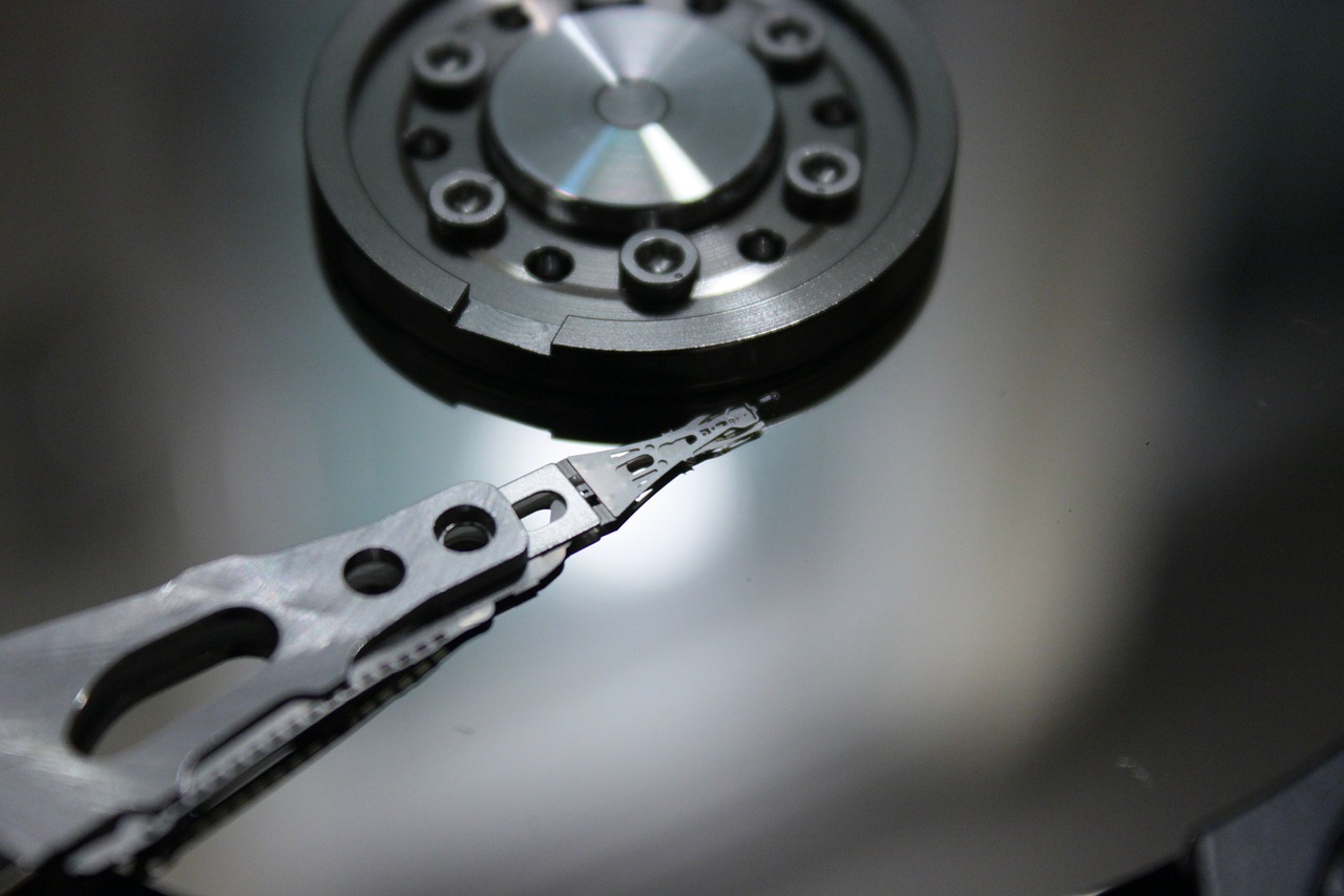
A hard disk drive consists of a set of one or more platters, which are disks of non-magnetic material such as aluminium. The platters spin at a constant speed on a common axle which we call a spindle – and by extension we often refer to the entire hard drive unit as a spindle too. The platters are coated in a thin layer of ferromagnetic material, which is where data is stored in binary form in concentric circles which we call tracks. Each track is divided into equal-sized segments called sectors and it is these that hold the data, along with additional overheads such as error correction codes. Traditionally, a sector contained 512 bytes of user data – but modern disks conforming to the Advanced Format standard use 4096 bytes for a sector. Data is read and written by a read/write head located on the end of a movable actuator arm which can traverse the platter – and of course with multiple and/or double-sided platters there will be multiple heads.

That’s where disk’s superpowers came from: the winning combination of a moving head and the concentric tracks of data. These days it almost seems like a flaw, but to appreciate the magic you need to consider the technology that disk replaced.

The Bad Old Days

Before disk, we had tape – a medium still in use today for other purposes such as backups. A big spinning reel of magnetic tape can transfer data in and out pretty fast (i.e. it has a high bandwidth) when the I/O is sequential, because the blocks are stored contiguously on the tape. But any kind of random I/O requires a mechanical delay (i.e. high latency) as the tape is wound backwards or forwards to locate the starting block and place it in front of the fixed read/write head. The time taken to locate the starting block is known as the seek time – a term that has haunted storage for decades.

When disk arrived it seemed revolutionary (pardon the pun). Like tape, disk used spinning magnetic media, but unlike tape, the read/write head could now move – allowing drastically reduced seek times. Want to move from reading the last sector on the disk to the first? No problem, the actuator arm simply moves across the tracks and then the platter rotates to find the first sector. A tape, on the other hand, would need to rewind the entire reel.

So, ironically, disk represented a massive leap forward for the performance of random I/O. How the mighty have fallen… but I’m going to save any talk of performance until the next post. For now, we need to finish off describing the basic layout of disk.

On The Edge

The picture on the right shows a traditional disk layout, where individual sectors (C) spread out across tracks (A) in the same way as a slice of cake or pie. If you consider a set of sectors (B – all those shaded in blue) you can see that they get longer the further towards the edge they get. How long does it take to read three consecutive sectors on a track, such as those highlighted green (D)? In the diagram those three sectors cover 90 degrees of the platter, so the time to read them would be one quarter of a revolution. And crucially, that would be the same no matter how far in or out they were from the edges.

In this traditional model, each sector contains the same amount of data (512 or 4096 bytes plus overheads). Since data is nothing more than bits (zeros and ones) we can say that the density of those bits is greater towards the centre of the platter and lower at the edge. In other words, we aren’t really utilising all of the available platter surface as we move further towards the edge. This directly affects the capacity of the drive, since less data is being stored than the platter can physically allow. There are solutions to this, however – and the most common solution is zoned bit recording.

In The Zone

To ensure that all of the available surface is used on each platter, many modern disk drives used a technique where the number of sectors per “slice” increases towards the edge of the disk. To simplify this design, tracks are placed into zones, each of which has a defined number of sectors per track. The result is that outer zones squeeze more sectors on to each track than inner zones. This has the benefit of increasing the capacity of the drive, because the surface is more efficiently used and bit densities remain consistently high.

But zoned bit recording also has another interesting effect: on the outer edge, more sectors now pass under the head per revolution. To put that more simply, the outer edge has a higher transfer rate (i.e. bandwidth) than the inner edge. And since most drives tend to number their tracks starting at the outer edge and working inwards, the result is that data stored at the logical start of a drive benefits from this higher bandwidth while data stored at the end experiences the opposite effect.

This is nothing to do with latency though, this is purely a bandwidth phenomenon. Latency is a whole different discussion – and as such, the subject of a whole different post…

The Most Expensive CPUs You Own

Storage for DBAs: Take a look in your data centre at all those humming boxes and flashing lights. Ignore the storage and networking gear for now and just concentrate on the servers. You probably have many different models, with different types and numbers of CPUs and DRAM inside. My question is, which CPUs are the most expensive? Almost without exception, the answer will be the CPUs inside your database servers…

In the last couple of posts I talked about the real cost of enterprise database software in general and Oracle RAC in particular. The point I was making was that database software, which is traditionally licensed by the CPU core, is expensive in comparison to the cost of the hardware on which it runs. But since the hardware fundamentally affects the performance – and therefore value for money – of the software, it’s important to make the right choices when building a database system. And yes, predictably, I believe that this means using flash memory instead of disk – but don’t worry, that’s not the main message behind post.

Lawn Mower Tax

Think of any consumer item which comes in multiple sizes and price brackets. I don’t know, let’s say a lawn mower. To simplify, let’s assume you can buy three different types of mower: small ($250), medium ($500) and large ($1000). The small one is cheaper but less powerful, so it takes longer to cut your grass, while the large one is the most expensive but requires the shortest amount of time. Which would you pick?

There’s no right answer because it depends on your requirements. But let’s introduce an unexpected complication into the mix: lawn mower tax. The government, in their wisdom, imposes a $50,000 tax on the purchase of any new lawn mower regardless of size. You still need a mower so you are forced to pay the tax, but is your choice influenced? The chances are you would buy the larger model, because a) the percentage difference in overall price is much less, and b) it avoids the risk of needing to upgrade in the future and having to pay the tax again. The $51,000 large mower represents better value for money than the two smaller models.

CPU Tax

You can think of database software in the same way. There are countless types of CPU available on the market right now: Intel, AMD, ARM, IBM Power, Oracle / Fujitsu SPARC, etc. Each vendor has many models and architectures, clock speeds and power ratings, yet they all share one important property: core count. And that core count is subject to the massive “CPU tax” that is the database software license. I’m sticking to the Oracle Database in this post but the same applies to Microsoft SQL Server (where licenses are core-based from SQL2012 onwards), Sybase and so on.

Take a standard two-socket sixteen-core Intel Xeon-based server as an example: there are a multitude of CPU models fitting that description. Even if we restrict ourselves to the Sandy Bridge-EP range Wikipedia shows there are 11 different models fitting the description of “8 cores per socket”. Yet not all CPUs are equal. Wouldn’t it make sense, given the massive cost associated with core-based licensing, so ensure you are using the processor which gives you the best performance, i.e. value for money, per license?

Performance Per Licenseable Core

The problem of determining which CPUs provide the best value for money was one I struggled with for a while. Looking at benchmarks like SPECint and the datasheets from Intel and co, it’s hard not to be overwhelmed by data – and if I’m honest I probably don’t have the systems-level knowledge to interpret it accurately. Ironically, the solution came from someone who does have that knowledge, but showed me that it isn’t required because there’s a much simpler way. More importantly, benchmarks like SPECint don’t take into account what we want these CPUs to do, which is to run the Oracle Database.

Kevin Closson‘s elegant and annoyingly simple solution was to use TPC benchmarks – specifically the transactional TPC-C benchmark from Oracle databases, results from which are freely available here. All we need to do then is simply download the spreadsheet, filter out the non-Oracle workloads and then divide the value of tpmC (the number of orders that can be fully processed per minute) by the number of CPU cores to get the performance per core.

Since this is an Oracle-specific calculation we also then need to multiply this by Oracle’s Processor Core Factor (see link on this page) to get the ultimate figure we need to know, the performance per license. Here’s my working copy of the spreadsheet, but I make no claims to its accuracy and will not keep this screenshot up-to-date. You should recalculate every time you want to make a judgement on which servers to use, it’s a very simple exercise.

Click to enlarge — Performance per licensable core (based on published TPC-C benchmark results using Oracle) – click to enlarge

The red column is the performance per licenseable core, marked “Perf / license“. Hopefully it’s obvious that this is just a re-work of Kevin’s ideas, many of which he posted in this blog article, which I highly recommend reading. As such I can claim no credit, except for any mistakes.

The Flash Angle

Of course, this wouldn’t be a flashdba article without some mention of flash memory. As discussed above there are many different types and models of CPU, but there is one great leveller: CPUs are all equally good at doing nothing. If your processors are waiting on I/O then they are not working – and that has a direct negative effect on the value you are realising from them.

In the above chart, the last benchmark result (with the best value for performance per licensable core) is this one performed by Cisco. Now, I honestly didn’t engineer this article to work out this way, but it so happens that Cisco used a pair of Violin Memory 6616 flash memory arrays to achieve this workload. (I’d almost* be happier if this had been a competitor’s flash array, because I don’t want this to look like an advert for my employer and therefore detract from my point…)

The point I’m aiming to make here is that it’s worth using the best-performing processors in order to see value for money from your database licenses. But to enable that, the processors need to be released from the chains of high-latency storage – and that, quite simply, means using flash.

* almost, but not quite

OOW13: The Future Is Here (Just Don’t Mention “Legacy”)

Last week I attended Oracle OpenWorld 2013 in the stunning city of San Francisco, along with 60,000 other attendees. At times it felt like we’d taken over the entire city, with every street, bus, billboard and hotel plastered in Oracle logos and pictures of engineered systems… although apparently there was some other stuff going on too.

I learnt a lot from OOW this year. I met many customers and potential customers, attended sessions from Oracle and its partners (including Violin’s competitors) and spent some time with friends at OaktableWorld as an antidote to the marketing hype. Oracle is many things to many people, but one thing that’s hard to deny is the company’s drive for innovation. Every year there are new products, new features, new options to learn – it’s very impressive. Of course, each one of these invariably means paying more license money – but those yachts don’t come cheap. This year as we looked to the future there were discussions about In Memory, Big Data, the Internet of Things and M2M. But what about the present? And more importantly, what about those of us still tied to the past?

The Database In Memory Option

In his opening keynote this year, Larry Ellison announced the Oracle Database In Memory Option, seen by many as an attempt to counter SAP’s HANA In-Memory database and Microsoft’s In Memory OLTP option for SQL Server 2014. This was by no means the only announcement of the week, or even the night (take, for example, the Oracle Big Memory Machine which, with 384 cores, I can’t help feeling would have been better named the Big License Bill Machine), but it’s a great example of the problem I want to discuss.

The obvious criticism is Oracle’s tiresome policy of pre-announcing and re-announcing the same thing (perfectly described by Doug Henschen here). The In-Memory Option isn’t available yet, nor will it be until “sometime next year”, which could conceivably be after OpenWorld 2014. But my real issue is that, like many other announcements, it’s a feature of the 12c database… which means almost everyone running in production won’t be able to use it.

Ok so maybe by the time Oracle finally rolls it out there will be some early adopters running 12c on their critical systems. But as the saying goes, you can always spot the pioneers by the arrows sticking out of their backs. Many people will refuse to upgrade to Oracle 12c until at least the release of version 2. And many, many more people simply won’t have a choice. We all spent a week talking about new or unreleased features that will change our lives, but how many customers will use them in production before next year’s slew of announcements?

Legacy Applications

The majority of organisations that I speak to are running legacy applications to support their businesses. The more risk-averse the business, the more ancient and convoluted the applications being supported (which is ironic if you consider the risk associated with maintaining old, complex code). Speak to any bank or telco and you’ll find applications from the previous decade running on versions of Oracle (or MSSQL, Sybase, etc) that you’d almost forgotten about. Scratch the surface and you’ll find lots of stuff on 11g Release 2, lots on 11gR1, plenty of stuff on 10.2 and maybe even 10.1. Dig really deep and horror of horrors, 9i is only just the beginning.

Not only that, but you’ll often find these databases aren’t even running on the terminal (i.e. supported) patchset! Why? Because upgrading an application or a database is a mammoth task, filled with risk and cost. I know I’m not the only one that has worked on 18+ month database upgrade projects which never even tasted success. Even applying a patchset requires full regression testing of an application – and if it’s a legacy application what are the support implications?

legacy-risk-stack — List of Legacy Refresh tasks in order of increasing risk and time/cost

In my view, despite all the talk of new technologies and paradigm shifts, the need to refresh legacy applications is more relevant now than ever. I guess I see it more working for a company like Violin because replacing legacy storage with flash memory offers a massive win with relatively little risk. Upgrading to 12c, on the other hand, is not a project to be treated lightly – despite the promises of features such as the Database In Memory option. Many customers simply cannot afford the time, money or risk associated with upgrades and migrations, despite any potential rewards. Yet who is championing them?

Footnote

I’m excited and intrigued by the new product launched by my employer Violin Memory, the Force 2510 Memory Appliance. I don’t usually use my blog to directly promote our products but this one interests me because it fits in below the list in the above picture, offering memory speeds without application or database changes. I hope to get one in my lab soon so I can blog what I see…

The Real Cost of Oracle RAC

Storage for DBAs: In my previous article (in this mini-series on database economics) I explained how to calculate the cost of a mid-range Oracle database system. My motive was a concern that many people working either directly or indirectly with database software are uninformed about just how expensive it is – particularly in comparison to the cost of hardware. And in this article I want to cover the great granddaddy of Oracle licenses costs: Oracle Real Application Clusters (RAC).

I also want to show you a little-known trick that can allow you to build a two-node fully active/active RAC cluster for a fraction of the price you would normally expect to pay.

But first, let’s talk about RAC…

Oracle RAC: High Availability For the Masses

There was a time, long ago, when big servers were very expensive. Many people ran Oracle on RISC-based UNIX systems, which had limited scalability in terms of the number of CPU cores and the maximum amount of physical memory. Oracle recognised this scalability issue and built a software solution for it, initially called Oracle Parallel Server (OPS). If you never used OPS in anger you should ask some of the grizzled, battle-scarred veterans who did how they fared against it, but at least in theory it allowed customers to scale out when scaling up wasn’t really possible.

However, things change – and nowhere more so than in IT. The days of big iron RISC systems seem long ago and nowadays (comparatively) cheap multicore x86 hardware is the norm. Scaling up to 80 cores in a server is not unusual, so the need for a software scalability solution is less strong than it was. However, Oracle knows a thing or two about staying at the top, so OPS became Real Application Servers and the scalability marketing message got overtaken by a new claim: high availability. Yes, Oracle RAC allows you to run one database across multiple nodes so if you look at it the right way that’s increasing system availability.

Of course, If you look at it another way (as I do), increasing the number of nodes is actually increasing the risk of failure to a single node. Plus, adding a whole raft of cluster functionality such as cache coherence, cluster filesystems and cluster ready services is just adding complexity, which is the enemy of availability. Yet everyone in the RAC game lives with the same shared deception: that losing a whole node does not count as a service outage. Sure, you get a whole load of users that get kicked off. Ok, so you have to bounce a whole set of application servers. But hey, technically it wasn’t a full outage so the SLAs weren’t affected. Er… ok… I think I’ve made my thoughts clear on this before.

Oracle RAC: The Expensive Way

There are two reasons why RAC can be expensive, or to put it another way two dimensions. The price goes up as the license cost increases, but it also goes up in multiples as the architecture scales out to multiple nodes.

In general, RAC is a feature of Oracle Enterprise Edition – in fact looking at the prices on the Oracle Store as I write this it’s the joint-most-expensive option (along with Oracle OLAP) priced at $23k per core (list)… If you consider that the Enterprise Edition license is $47.5k per core then that’s nearly half as much again. Don’t forget that Oracle’s core multiplication factor table determines that we need to multiply these costs by 0.5 for Intel Xeon processors, which is what I’m using in this example (see the first article in this series if you don’t know what this means).

Let’s state some assumptions for this imaginary Oracle RAC cluster we are building. It will have 4 nodes (16 cores per node) and 20TB of usable disk storage. We’ll also assume that in buying the licenses we got a 60% discount. We’re looking at the three-year price and, as always, the maintenance costs us 22% of the net license cost. I’m including the Oracle Diagnostics Pack ($5k per core) in the license cost too – surely nobody can cope without it these days?

The total cost over three years, just for hardware, software and support (i.e. discounting TCO-type calculations like power, cooling, etc) is now up at £1.8m. That’s a relatively large amount of money! But what I find really interesting is the proportion that goes to the database vendor compared to the proportion that is spent on hardware:

The storage (which I naturally have an interest in) is just 8% of the total cost, while the database vendor’s products and support services comprise 89% of the total cost. This is where database consolidation starts to make sense (more databases on the same hardware means better value for money from the core-based licenses). It’s also where flash memory storage makes sense, because it allows a far better return on this massive investment: firstly by unleashing applications to run at the speed of memory, and secondly by unlocking (expensive) CPUs which are otherwise stuck waiting on I/O from slow disk storage systems.

Oracle RAC: The Inexpensive Way

But wait, I promised you an alternative to the costly system above. What is it? The answer can be found buried deep within Oracle’s Software Investment Guide (page 11 of the current published version) where we find the following information: from Oracle 10g onwards, Oracle Standard Edition includes the Real Application Clusters Option provided customers use Oracle Clusterware and ASM. Since Standard Edition is limited to a maximum of 4 CPU sockets (not cores!!) this effectively means a two-node system using two-socket servers.

That’s still an amazing revelation – it’s basically RAC (with certain caveats) for free! With the right choice of high-end CPU, a two-socket server can deliver massive performance. Let’s have a look at the cost of a two-node RAC system running on Standard Edition using the same assumptions from above [massive thanks to Doug (see comments below) for pointing out my mistake – now corrected – that Standard Edition is licensed by the socket not the core and that the core multiplication factor therefore does not apply]:

Now many people will think, “Hang on I can’t cope without Enterprise Edition” … but for this level of saving, isn’t it worth giving that some closer analysis? The real bonus here is that, in only paying licenses by the socket, you can achieve a massive benefit if you use the fastest processors with the largest number of cores and not pay any penalty.

The price of Standard Edition RAC is 87% of the price of our previous configuration. (If you were to compare a like-for-like scenario where 2 node Enterprise Edition RAC moved to 2 node Standard Edition RAC the saving would instead be £702.5k or 76%)

Conclusion

Everything here is just speculation, based on the information available from Oracle at the time of writing. You should not construe my remarks as guarantees or facts, but instead do your own research and talk to your local database vendor’s representatives.

The point of writing this article is that technical people don’t always have a handle on price, because in some organisations they don’t always need to. But when the technical design has such a dramatic effect on the price, I think we all ought to be looking at the bigger picture and taking the time to work out the implications of our choices.

Software, as they say in Redwood Shores, doesn’t come cheap…

The Real Cost of Enterprise Database Software

Storage for DBAs: The strange thing about enterprise databases is that the people who design, manage and support them are often disassociated from the people who pay the bills. In fact, that’s not unusual in enterprise IT, particularly in larger organisations where purchasing departments are often at opposite ends of the org chart to operations and engineering staff.

I know this doesn’t apply to everyone but I spent many years working in development, operations and consultancy roles without ever having to think about the cost of an Oracle license. It just wasn’t part of my remit. I knew software was expensive, so I occasionally felt guilt when I absolutely insisted that we needed the Enterprise Edition licenses instead of Standard Edition (did we really, or was I just thinking of my CV?) but ultimately my job was to justify the purchase rather than explain the cost.

On the off chance that there are people like me out there who are still a little bit in the dark about pricing, I’m going to use this post to describe the basic price breakdown of a database environment. I also have a semi-hidden agenda for this, which is to demonstrate the surprisingly small proportion of the total cost that comprises the storage system. If you happen to be designing a database environment and you (or your management) think the cost of high-end storage is prohibitive, just keep in mind how little it affects the overall three-year cost in comparison to the benefits it brings.

Pricing a Mid-Range Oracle Database

Let’s take a simple mid-range database environment as our starting point. None of your expensive Oracle RAC licenses, just Enterprise Edition and one or two options running on a two-socket server.

At the moment, on the Oracle Store, a perpetual license for Enterprise Edition is retailing at $47,500 per processor. We’ll deal with the whole per processor thing in a minute. Keep in mind that this is the list price as well. Discounts are never guaranteed, but since this is a purely hypothetical system I’m going to apply a hypothetical 60% discount to the end product later on.

I said one or two options, so I’m going to pick the Partitioning option for this example – but you could easily choose Advanced Compression, Active Data Guard, Spatial or Real Application Testing as they are all currently priced at $11,500 per processor (with the license term being perpetual – if you don’t know the difference between this and named user then I recommend reading this). For the second option I’ll pick one of the cheaper packs… none of us can function without the wait interface anymore, so let’s buy the Tuning Pack for $5,000 per processor.

The Processor Core Factor

I guess we’d better discuss this whole processor thing now. Oracle uses per core licensing which means each CPU core needs a license, as opposed to per socket which requires one license per physical chip in the server. This is normal practice these days since not all sockets are equal – different chips can have anything from one to ten or more cores in them, making socket-based licensing a challenge for software vendors. Sybase is licensed by the core, as is Microsoft SQL Server from SQL 2012. However, not all cores are equal either… meaning that different types of architecture have to be priced according to their ability.

The solution, in Oracle’s case, is the Oracle Processor Core Factor, which determines a multiplier to be applied to each processor type in order to calculate the number of licenses required. (At the time of writing the latest table is here but always check for an updated version.) So if you have a server with two sockets containing Intel Xeon E5-2690 processors (each of which has eight cores, giving a total of sixteen) you would multiply this by Oracle’s core factor of 0.5 meaning you need a total of 16 x 0.5 = 8 licenses. That’s eight licenses for Enterprise Edition, eight licenses for Partitioning and eight licenses for the Tuning Pack.

What else do we need? Well there’s the server cost, obviously. A mid-range Xeon-based system isn’t going to be much more than $16,000. Let’s also add the Oracle Linux operating system (one throat to choke!) for which Premier Support is currently listing at $6,897 for three years per system. We’ll need Oracle’s support and maintenance of all these products too – traditionally Oracle sells support at 22% of the net license cost (i.e. what you paid rather than the list price), per year. As with everything in this post, the price / percentage isn’t guaranteed (speak to Oracle if you want a quote) but it’s good enough for this rough sketch.

Finally, we need some storage. Since I’m actually describing from memory an existing environment I’ve worked on in the past, I’m going to use a legacy mid-range disk array priced at $7 per GB – and I want 10TB of usable storage. It’s got some SSD in it and some DRAM cache but obviously it’s still leagues apart from an enterprise flash array.

Price Breakdown

That’s everything. I’m not going to bother with a proper TCO analysis, so these are just the costs of hardware, software and support. If you’ve read this far your peripheral vision will already have taken in the graph below. so I can’t ask you to take a guess… but think about your preconceptions. Of the total price, how much did you think the storage was going to be? And how much of the total did you think would go to the database vendor?

The storage is just 17% of the total, while the database vendor gets a whopping 80%. That’s four-fifths… and they don’t even have to deal with the logistics of shipping and installing a hardware product!

Still, the total price is “only” $430k, so it’s not in the millions of dollars, plus you might be able to negotiate a better discount. But ask yourself this: what would happen if you added Oracle Real Application Clusters (currently listing at $23,000 per processor) to the mix. You’d need to add a whole set of additional nodes too. The price just went through the roof. What about if you used a big 80-core NUMA server… thereby increasing the license cost by a factor of five (16 cores to 80)? Kerching!

Performance and Cost are Interdependent

There are two points I want to make here. One is that the cost of storage is often relatively small in terms of the total cost. If a large amount of money is being spent on licensing the environment it makes sense to ensure that the storage enables better performance, i.e. results in a better return on investment.

The second point is more subtle – but even more important. Look at the price calculations above and think about how important the number of CPU cores is. It makes a massive difference to the overall cost, right? So if that’s the case, how important do you think it is that you use the best CPUs? If CPU type A gives significantly better performance than CPU type B, it’s imperative that you use the former because the (license-related) cost of adding more CPU is prohibitive.

Yet many environments are held back by CPUs that are stuck waiting on I/O. This is bad news for end users and applications, bad news for batch jobs and backups. But most of all, this is terrible news for data centre economics, because those CPUs are much, much more expensive than the price you pay to put them in the server.

There is more to come on this subject…

Storage Myths: Put Oracle Redo on SSD

Storage for DBAs: “My database is slow”… “Well then why not put your redo logs on SSDs?” Gaaaah. I still hear people having this discussion and it drives me mad. “Nobody got fired for putting Oracle redo on …<flash vendor>”. Yeah right, but does that mean it was worth the investment?

I’m bored of this line of illogical “reasoning”, so here are three reasons why you shouldn’t put your redo logs on SSD.

1. Solve The Right Problem

If a database is slow, find out why. Investigate, troubleshoot, resolve. Don’t throw hardware at it without understanding what the problem is. Redo is written by the Oracle Log Writer process – and the wait event log file parallel write covers the writing of redo records from the log buffer into the online redo log files. If you are seeing high average wait times for log file parallel write (or occasional high wait times in the Wait Event Histogram) maybe it’s time to investigate the speed of redo I/Os. Otherwise … leave it alone, or you are fixing the wrong issue.

Also, let’s not confuse the wait event log file sync with log file parallel write. Log file sync is experienced by foreground processes waiting on the log writer to complete a flush of the log buffer to storage. It’s tempting to assume high log file sync times are therefore a consequence of slow log writes, but as Kevin Closson points out in this must-read article, most log file sync waits are actually processing issues where the log writer is not getting enough CPU time.

2. SSD Write Performance Sucks

Huh? You thought I was pro-SSD right? Ok so I’m being a bit crafty, because the terms SSD and Flash are not really synonymous. SSD stands for Solid State Disk (or Device depending on who you ask), which generally means a set of flash chips crafted into the shape of a hard disk drive and plugged into a HDD-shaped hole somewhere via the use of a Flash Memory Controller. This interface takes page-based flash memory and makes it look like block-based storage – and each SSD in an array has its own controller.

There is a fundamental difference between an all-flash array and a set of SSDs masquerading as disks: an all-flash array can manage the flash holistically while the SSD-populated array cannot. This matters because flash is awkward to work with – for example, flash pages must be erased before they are written to – a process which is both slow and cumbersome, since other pages are locked (even from reads) during an erase.

The all-flash array is able to avoid the consequences of these restrictions by managing the flash globally, so that erases do not block reads and writes. In contrast, SSDs shoved into a disk array cannot communicate with each other to indicate when they are busy performing this garbage collection process, resulting in unpredictable performance and horrible spikes in latency as I/Os queue up behind the erase process.

3. Disk Is Good Enough

You didn’t expect me to say that, did you? Don’t get me wrong, disk is terrible at random I/O. Really, truly awful. But here’s the thing: the Oracle log writer performs large, sequential writes. And disk is ok with sequential I/O, particularly if you are using faster spindles like the 15k RPM drives.

Flushing the log buffer to storage involves writing some multiple of the redo log block size (512 byte default but configurable to 1024 or 4096 bytes from Oracle version 11.2). If your system is busy enough that you believe you have redo performance issues, it seems likely that those writes will be larger as more redo is created per log flush. The larger the write, the more efficient it will be on disk as the impact of the initial seek time is averaged out.

But hey, don’t take my word for it. Trust the evidence – and it turns out there is a wealth of data out there for anyone to analyse… right here: http://www.tpc.org/

The thing about TPC-C benchmarks is that they generate redo logs like you wouldn’t believe. So if anyone needs the ultimate redo performance it’s a system like this one, which set a world record back in September 2012 (which Oracle crowed about in it’s usual classy way by using it to bash IBM). The great thing about TPC results is that they come with a complete full disclosure report so you can see just how the vendors did it. And in the full disclosure report for this submission, where was the redo located? On a RAID set consisting of 600GB 15K RPM disk drives (see page 21). If disk is fast enough for a world record, it’s fast enough for you.

Incidentally, the datafiles in that benchmark were located on 2x Violin Memory 6616 arrays – which also tells you something important: if you are migrating from disk to flash, the first thing you need to move is the primary data, not the redo.

The Counter-Argument: Flash is Not SSD

Now I don’t want to wrap this article up giving you the impression that you shouldn’t move your redo logs to flash memory, so I’ll leave you with some counter arguments to the above. When I build a database, I always put the redo logs on flash (not on SSD mind, but on a flash memory array). Here’s why:

1. Violin Isn’t Limited By Writes

I know, I know … that sounds like a sales pitch. I usually try to talk about flash in general, which is why I originally wrote “All-flash arrays aren’t limited by writes”, but the truth is I don’t know other all-flash arrays to the extent that I know Violin… so forgive me for sticking with what I know.

I’ll explain Violin’s methods for guaranteeing sustained ultra-low write latency some other day. for now, let’s just see the evidence:

Load Profile              Per Second    Per Transaction
~~~~~~~~~~~~         ---------------    ---------------
      DB Time(s):              197.6                2.8
       DB CPU(s):               18.8                0.3
       Redo size:    1,477,126,876.3       20,568,059.6
   Logical reads:          896,951.0           12,489.5
   Block changes:          672,039.3            9,357.7
  Physical reads:           15,529.0              216.2
 Physical writes:          166,099.8            2,312.8

That’s over 1.4GB/sec of sustained redo generation from a 5 minute snapshot (see this post for details) using just a single Violin Memory 6616 array connected over 8Gb fibre channel. The AWR snapshot was 5 minutes long but the workload had been running for an extended period prior to the capture. Don’t leave here with the illusion that redo on flash memory isn’t blindingly fast.

2. Your First Design Goal Should Be Simplicity

There is a quote often attributed to Albert Einstein which says, “Everything should be made as simple as possible, but no simpler“. This applies perfectly to system design – and is one reason why I always recommend an all-flash database design over a flash and disk hybrid. Yes it’s possible to put some datafiles here and others over there, redo logs on disk and primary data on flash, etc. But the simplest design is to put everything on high performance, low latency flash. Is it the cheapest solution? Maybe not always on list price, but it probably will be based on TCO.

Conclusion

Look, if you want to put your redo logs on flash, I’m not going to argue. I’m not saying that it’s a bad thing.

What is a bad thing though is the practice of taking a disk-based database and sticking some SSDs in to home the redo logs. That’s just silly. The first part of the database you should move to flash is the primary data. If it makes sense to relocate the whole database (which it almost always does, because that disk array doesn’t belong in your data centre anymore – it belongs in a museum) then go for it. Just don’t compromise on having only the redo logs on flash or SSD, because then you have essentially built yourself an anti-TPC-C benchmarking system! And what’s the opposite of a system that goes really fast…?

7 Steps to Guarantee People Will Read Your Posts

I see this type of article pop up all the time on places link LinkedIn and SlideShare. Here’s my response…

Chess is a suitably abstract subject and so can seem relevant to anything

Choose an arbitrary number of items, e.g. 7
Combine this with a suitable noun that the number will describe, e.g. steps, tips, ways, methods etc
Make sure you put this combination at the start of your article’s title to entice people to read your post. The number draws people in with the promise of a finite solution, neatly packaged and ready for consumption.
Offering some kind of vague promise helps, e.g. the use of words like “guarantee” or “master”. Alternatively, imply that superior beings to your readers already know this information, e.g. “The 4 Things That Brilliant People During Breakfast”. In this way you imply that you are letting your readers in on a magical secret they can never otherwise know. To reach the ultimate low, suggest that someone no longer with us would have done this, e.g. Steve Jobs.
Choose a random picture to head the article up. This doesn’t have to be relevant but it does have to be high quality. Be careful not to use something owned by someone else (I use public domain images from Pixabay). Abstract pictures like pieces on a chess board will have your readers wondering about the significance or trying to count the pieces to see if they correspond to the arbitrary number in the title.
Don’t worry if you can’t actually hit the number of items you promised in the title, because by then people will already have clicked through to your site. And traffic is all that matters, right?

Come on people, can we get some decent content and stop all this nonsense?