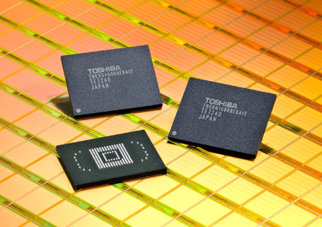
Understanding Flash: SLC, MLC and TLC

The last post in this series discussed the layout of NAND flash memory chips and the way in which cells can be read and written (programmed) at the page level but have to be erased at the (larger) block level. I finished by mentioning that erase operations take substantially longer than read or program operations… but just how big is the difference?

Knowing the answer to this involves first understanding the different types of flash memory available: SLC, MLC and TLC.

Electrons In A Bucket?

Whenever I’ve seen anyone attempt to explain this in the past, they have almost always resorted to drawing a picture of electrons or charge filling up a bucket. This is a terrible analogy and causes anyone with a deep understanding of physics to cringe in horror. Luckily, I don’t have a deep understanding of physics, so I’m going to go right along with the herd and get my bucket out.

A NAND flash cell, i.e. the thing that stores a value of one or zero, is actually a floating gate transistor. Programming the cell means putting electrons into the floating gate, causing it to become (negatively) charged. Erasing the cell means removing the electrons from the floating gate, draining the charge. The amount of charge contained in the floating gate can be varied from zero up to a maximum value – this is an analogue system so there is no simple FULL or EMPTY state.

Because of this, the amount of charge can be measured and thresholds assigned to indicate a binary value. What does that mean? It means that, in the case of Single Level Cell (SLC) flash anything below 50% of charge can be considered to be a bit with a value of 1, while anything above 50% can be considered a bit with a value of 0.

But if i decided to be a bit more careful in the way I fill or empty my bucket of charge (sorry), I could perhaps define more thresholds and thus hold two bits of data instead of one. I could say that below 25% is 11, from 25% to 50% is 10, from 50% to 75% is 01 and above 75% is 00. Now I can keep twice as much data in the same bucket. This is in fact Multi Level Cell (MLC). And as the picture shows, if I was really careful in the way I treated my bucket, I could even keep three bits of data in there, which is what happens in Three Level Cell (TLC):

The thing is, imagine this was a bucket of water (comparing electrons to water is probably the last straw for anyone reading this who has a degree in physics, so I bid you farewell at this point). If you were to fill up your bucket using the SLC method, you could be pretty slap-dash about it. I mean it’s pretty obvious when the bucket is more than half full or empty. But if you were using a more fine-grained method such as MLC or TLC you would need to fill / empty very carefully and take exact measurements, which means the act of filling (programming) would be a lot slower.

To really stretch this analogy to breaking point, imagine that every time you fill your bucket it gets slightly damaged, causing it to leak. In the SLC world, even a number of small leaks would not be a big deal. But in the MLC or (especially) the TLC world, those leaks mean it would quickly become impossible to keep using your bucket, because the tolerance between different bit values is so small. For similar reasons, NAND flash endurance is greatly influenced by the type of cell used. Storing more bits per cell means a lower tolerance for errors, which in turn means that higher error rates are experienced and endurance (the number of program/erase cycles that can be sustained) is lower.

Timing and Wear

Enough of the analogies, let’s look at some proper data. The chart below uses sample figures from AnandTech:

You can see that as the number of bits per cell increases, so does the time taken to perform read, program (i.e. write) and erase operations. Erases in particular are especially slow, with values measured in milliseconds instead of microseconds. Given that erases also affect larger areas of flash than reads and programs, you can start to see why the management of erase operations on flash is critical to performance.

Also apparent on the chart above is the massive difference in the number of program / erase cycles between the different flash types: for SLC we’re talking about orders of magnitude in difference. But of course SLC can only store one bit per cell, which means it’s much more expensive from a capacity perspective than MLC. TLC, meanwhile, offers the potential for great value for money, but none of the performance requirements you would need for tier one storage (although it may well have a place in the world of backups). It is for this reason that MLC is the most commonly used type of flash in enterprise storage systems. (By the way I’m so utterly disinterested in the phenomena of “eMLC” that I’m not going to cover it here, but you can read this and this if you want to know more on the subject…)

Warning: Know Your Flash

One final thing. When you buy an SSD, a PCIe flash card or, in the case of Violin Memory, an all-flash array you tend to choose between SLC and MLC. As a very rough rule of thumb you can consider MLC to be twice the capacity for half the performance of SLC, although this in fact varies depending on many factors. However there are some all flash array vendors who use both SLC and MLC in a sort of tiered approach. That’s fine -and if you are buying a flash array I’m sure you’ll take the time to understand how it works.

But here’s the thing. At least one of these vendors insists on describing the SLC layer as “NVRAM” to differentiate from the MLC layer which it simply describes as using flash SSDs. The truth is that the NVRAM is also just a bunch of flash SSDs, except they are SLC instead of MLC. I’m not in favour of using educational posts to criticise competitors, but in the interest of bring clarity to this subject I will say this: I think this is a marketing exercise which deliberately adds confusion to try and make the design sound more exciting. “Ooooh, NVRAM that sounds like something I ought to have in my flash array…” – or am I being too cynical?

Update: January 2016

This article discusses what is known as 2D Planar NAND flash. Since publication, a new type of NAND flash called 3D NAND (led by Samsung’s branded V-NAND product) has become popular on the market. You can read about that here.

Understanding Flash: Blocks, Pages and Program / Erases

In the last post on this subject I described the invention of NAND flash and the way in which erase operations affect larger areas than write operations. Let’s have a look at this in more detail and see what actually happens. First of all, we need to know our way around the different entities on a flash chip (or “package“), which are: the die, the plane, the block and the page:

NAND Flash Die Layout (image courtesy of AnandTech)

Note: What follows is a high-level description of the generic behaviour of flash. There are thousands of different NAND chips available, each potentially with slightly different instruction sets, block/page sizes, performance characteristics etc.

• The package is the memory chip, i.e. the black rectangle with little electrical connectors sticking out of it. If you look at an SSD, a flash card or the internals of a flash array you will see many flash packages, each of which is produced by one of the big flash manufacturers: Toshiba, Samsung, Micron, Intel, SanDisk, SK Hynix. These are the only companies with the multi-billion dollar fabrication plants necessary to make NAND flash.
• Each package contains one or more dies (for example one, two, or four). The die is the smallest unit that can independently execute commands or report status.
• Each die contains one or more planes (usually one or two). Identical, concurrent operations can take place on each plane, although with some restrictions.
• Each plane contains a number of blocks, which are the smallest unit that can be erased. Remember that, it’s really important.
• Each block contains a number of pages, which are the smallest unit that can be programmed (i.e. written to).

The important bit here is that program operations (i.e. writes) take place to a page, which might typically be 8-16KB in size, while erase operations take place to a block, which might be 4-8MB in size. Since a block needs to be erased before it can be programmed again (*sort of, I’m generalising to make this easier), all of the pages in a block need to be candidates for erasure before this can happen.

Program / Erase Cycles

When your flash device arrives fresh from the vendor, all of the pages are “empty”. The first thing you will want to do, I’m sure, is write some data to them – which in the world of memory chips we call a program operation. As discussed, these program operations take place at the page level. You can then read your fresh data back out again with read operations, which also take place at the page level. [Having said that, the instruction to read a page places the data from that page in a memory register, so your reading process can in fact then selectively access subsets of the page if it desires – but maybe that’s going into too much detail…]

Where it gets interesting is if you want to update the data you just wrote. There is no update operation for flash, no undo or rewind mechanism for changing what is currently in place, just the erase operation. It’s a little bit like an etch-a-sketch, in that you can continue to turn the dials and make white sections of screen go black, but you cannot turn black sections of screen to white again without erasing the entire screen. An erase operation on a flash chip clears the data from all pages in the block, so if some of the other pages contain active data (stuff you want to keep) you either have to copy it elsewhere first or hold off from doing the erase.

In fact, that second option (don’t erase just yet) makes the most sense, because the blocks on a flash chip can only tolerate a limited number of program and erase options (known as the program erase cycle or PE cycle because for obvious reasons they follow each other in turn). If you were to erase the block every time you wanted to change the contents of a page, your flash would wear out very quickly.

So a far better alternative is to simply mark the old page (containing the unchanged data) as INVALID and then write the new, changed data to an empty page. All that is required now is a mechanism for pointing any subsequent access operations to the new page and a way of tracking invalid pages so that, at some point, they can be “recycled”.

Updating a page in NAND flash. Note that the new page location does not need to be within the same block, or even the same flash die. It is shown in the same block here purely for ease of drawing.

This “mechanism” is known as the flash translation layer and it has responsibility for these tasks as well as a number of others. We’ll come back to it in subsequent posts because it is a real differentiator between flash products. For now though, think about the way the device is filling up with data. Although we’ve delayed issuing erase operations by cleverly moving data to different pages, at some point clearly there will be no empty pages left and erases will become essential. This is where the bad news comes in: it takes many times longer to perform an erase than it does to perform a read or program. And that clearly has consequences for performance if not managed correctly.

In the next post we’ll look at the differences in time taken to perform reads, programs and erases – which first requires looking at the different types of flash available: SLC, MLC and TLC…

[* Technical note: Ok so actually when a NAND flash page is empty it is all binary ones, e.g. 11111111. A program operation sets any bit with the value of 1 to 0, so for example 11111111 could become 11110000. This means that later on it is still possible to perform another program operation to set 11110000 to 00110000 for example. Until all bits are zero it’s technical possible to perform another program. But hey, that’s getting a bit too deep into the details for our requirements here, so just pretend you never read this…]

Understanding Flash: What Is NAND Flash?

In the early 1980s, before we ever had such wondrous things as cell phones, tablets or digital cameras, a scientist named Dr Fujio Masuoka was working for Toshiba in Japan on the limitations of EPROM and EEPROM chips. An EPROM (Erasable Programmable Read Only Memory) is a type of memory chip that, unlike RAM for example, does not lose its data when the power supply is lost – in the technical jargon it is non-volatile. It does this by storing data in “cells” comprising of floating-gate transistors. I could start talking about Fowler-Nordheim tunnelling and hot-carrier injection at this point, but I’m going to stop here in case one of us loses the will to live. (But if you are the sort of person who wants to know more though, I can highly recommend this page accompanied by some strong coffee.)

Anyway, EPROMs could have data loaded into them (known as programming), but this data could also be erased through the use of ultra-violet light so that new data could be written. This cycle of programming and erasing is known as the program erase cycle (or PE Cycle) and is important because it can only happen a limited number of times per device… but that’s a topic for another post. However, while the reprogrammable nature of EPROMS was useful in laboratories, it was not a solution for packaging into consumer electronics – after all, including an ultra-violet light source into a device would make it cumbersome and commercially non-viable.

US Patent US4531203: Semiconductor memory device and method for manufacturing the same

A subsequent development, known as the EEPROM, could be erased through the application of an electric field, rather than through the use of light, which was clearly advantageous as this could now easily take place inside a packaged product. Unlike EPROMs, EEPROMs could also erase and program individual bytes rather than the entire chip. However, the EEPROMs came with a disadvantage too: every cell required at least two transistors instead of the single transistor required in an EPROM. In other words, they stored less data: they had lower density.

The Arrival of Flash

So EPROMs had better density while EEPROMs had the ability to electrically reprogram cells. What if a new method could be found to incorporate both benefits without their associated weaknesses? Dr Masuoka’s idea, submitted as US patent 4612212 in 1981 and granted four years later, did exactly that. It used only one transistor per cell (increasing density, i.e. the amount of data it could store) and still allowed for electrical reprogramming.

If you made it this far, here’s the important bit. The new design achieved this goal by only allowing multiple cells to be erased and programmed instead of individual cells. This not only gives the density benefits of EPROM and the electrically-reprogrammable benefits of EEPROM, it also results in faster access times: it takes less time to issue a single command for programming or erasing a large number of cells than it does to issue one per cell.

However, the number of cells that are affected by a single erase operation is different – and much larger – than the number of cells affected by a single program operation. And it is this fact that, above all else, that results in the behaviour we see from devices built on flash memory. In the next post we will look at exactly what happens when program and erase operations take place, before moving on to look at the types of flash available (SLC, MLC etc) and their behaviour.

NAND and NOR

To try and keep this post manageable I’ve chosen to completely bypass the whole topic of NOR flash and just tell you that from this moment on we are talking about NAND flash, which is what you will find in SSDs, flash cards and arrays. It’s a cop out, I know – but if you really want to understand the difference then other people can describe it better than me.

In the meantime, we all have our good friend Dr Masuoka to thank for the flash memory that allows us to carry around the phones and tablets in our pockets and the SD cards in our digital cameras. Incidentally, popular legend has it that the name “flash” came from one of Dr Masuoka’s colleagues because the process of erasing data reminded him of the flash of a camera. Presumably it was an analogue camera because digital cameras only became popular in the 1990s after the commoditisation of a new, solid-state storage technology called …