This is a very simple post to show the results of some recent testing that Tom and I ran using Oracle SLOB on Violin to determine the impact of using virtualization. But before we get to that, I am duty bound to write a paragraph of text featuring lots of long sentences peppered with industry buzz words. Forgive me, it’s just the way I’m wired.
It is increasingly common these days to find database environments running in virtual machines – even large, business critical ones. The driver is the trend to commoditize I.T. services and build consolidated, private-cloud style solutions in order to control operational expense and increase agility (not to mention reduce exposure to Oracle licenses). But, as I’ve said in previous posts, the catalyst has been the unblocking of I/O as legacy disk systems are replaced by flash memory. In the past, virtual environments caused a kind of I/O blender effect whereby I/O calls become increasingly randomized – and this sucked for the performance of disk drives. Flash memory arrays on the other hand can deliver random I/O all day long because… well, if you don’t know the reasons by now can I just recommend starting at the beginning. The outcome is that many large and medium-sized organisations are now building database-as-a-service platforms with Oracle databases (other database products are available) running in virtual machines. It’s happening right now.
Phew. Anyway, that last paragraph was just a wordy way of telling you that I’m often seeing Oracle running in virtual machines on top of hypervisors. But how much of a performance impact do those hypervisors have? Step this way to find out.
The Contenders
When it comes to running Oracle on a hypervisor using Intel x86 hardware (for that is what I have available), I only know of three real contenders:
Hyper-V has been an option for a couple of years now, but I’ll be honest – I have neither the time nor the inclination to test it today. It’s not that I don’t rate it as a product, it’s just that I’ve never used it before and don’t have enough time to learn something new right now. Maybe someday I’ll come back and add it to the mix.
In the meantime, it’s the big showdown: VMware versus Oracle VM. Not that Oracle VM is really in the same league as VMware in terms of market share… but you know, I’m trying to make this sound exciting.
The Test
This is going to be an Oracle SLOB sustained throughput test. In other words, I’m going to build an Oracle database and then shovel a massive amount of I/O through it (you can read all about SLOB here and here). SLOB will be configured to run with 25% of statements being UPDATEs (the remainder are SELECTs) and will run for 8 hours straight. What we want to see is a) which hypervisor configuration allows the greatest I/O bandwidth, and b) which hypervisor configuration exhibits the most predictable performance.
This is the configuration. First the hardware:
Violin Memory 6616 flash Memory Array
1x Dell PowerEdge R720 server
2x Intel Xeon CPU E5-2690 v2 10-core @ 3.00GHz [so that’s 2 sockets, 20 cores, 40 threads for this server]
128GB DRAM
1x Violin Memory 6616 (SLC) flash memory array [the one that did this]
8GB fibre-channel
And the software:
Hypervisor: VMware ESXi 5.5.1
Hypervisor: Oracle VM for x86 3.3.1
VM: Oracle Linux 6 Update 5 (with the Unbreakable Enterprise v3 Kernel 3.6.18)
Each VM is configured with 20 vCPUs and is using Linux Device Mapper Multipath and Oracle ASMLib. ASM is configured to use one single +DATA disgroup comprising 8 ASM disks (LUNs from Violin) with external redundancy. The database parameters and SLOB settings are all listed on the SLOB sustained throughput test page.
Results: Bare Metal (Baseline)
First let’s see what happens when we don’t use a hypervisor at all and just run OL6.5 on bare metal:
Ok so we’re looking at 1519 MB/sec of read throughput and 320 MB/sec of write throughput. Crucially, the lines are nice and consistent – with very little deviation from the mean. By dividing the amount of time spent waiting on db file sequential read(i.e. random physical reads) with the number of waits, we can calculate that the average latency for random reads was 438 microseconds.
Now we know what to expect, let’s look at the result from the hypervisor tests.
Results: VMware vSphere
VMware is configured to use Raw Device Mapping (RDM) which essentially gives the benefits of raw devices… read here for more details on that. Here are the test results:
Average read throughput for this test was 1133 MB/sec and write throughput averaged at 237 MB/sec. Average read latency was 596 microseconds. That’s an increase of 36%.
In comparison to the bare metal test, we see that total bandwidth dropped by around 25%. That might seem like a lot but remember, we are absolutely hammering this system. A real database is unlikely to ever create this level of sustained I/O. In my role at Violin I’ve been privileged to work on some of the busiest databases in Europe – nothing is ever this crazy (although a few do come close).
Results: Oracle VM
Oracle VM is based on the Xen hypervisor and therefore uses Xen virtual disks to present block devices. For this test I downloaded the Oracle Linux 6 Update 5 template from Oracle’s eDelivery site. You can see more about the way this VM was configured here. Here are the test results:
This time we see average read bandwidth of 1052MB/sec and average write bandwidth of 222MB/sec, with the average read latency at 607 microseconds, which is 39% higher than the baseline test.
Meanwhile, total bandwidth dropped by 31%. That’s slightly worse than VMware, but what’s really interesting is the deviation. Look at how ragged the lines are on the OVM test! There is a much higher degree of variance exhibited here than on the VMware test.
Conclusion
This is only one test so I’m not claiming it’s conclusive. VMware does appear to deliver slightly better performance than OVM in my tests, but it’s not a huge difference. However, I am very much concerned by the variance of the OVM test in comparison to VMware. Look, for example, at the wait event histograms for db file sequential read:
Wait Event Histogram
-> Units for Total Waits column: K is 1000, M is 1000000, G is 1000000000
-> % of Waits: value of .0 indicates value was <.05%; value of null is truly 0
-> % of Waits: column heading of <=1s is truly <1024ms, >1s is truly >=1024ms
-> Ordered by Event (idle events last)

                                                             % of Waits
                                          -----------------------------------------------
                                    Total
Hypervisor  Event                   Waits  <1ms  <2ms  <4ms  <8ms <16ms <32ms  <=1s   >1s
----------- ----------------------- ----- ----- ----- ----- ----- ----- ----- ----- -----
Bare Metal: db file sequential read 5557.  98.7   1.3    .0    .0    .0    .0
VMware ESX: db file sequential read 4164.  92.2   6.7   1.1    .0    .0    .0
Oracle VM : db file sequential read 3834.  95.6   4.1    .1    .1    .0    .0    .0    .0
The OVM tests show occasional results in the two highest buckets, meaning once or twice there were waits in excess of 1 second! However, to be fair, OVM also had more millisecond waits than VMware.
Anyway, for now – and for this setup at least – I’m sticking with VMware. You should of course test your own workloads before choosing which hypervisor works for you…
Thanks as always to Kevin for bringing Oracle SLOB to the community.
It’s that time of year again where lots of people write articles which begin with the words “It’s that time of year again…” and make endless references to crystal balls, tea leaves and the benefits of hindsight. But not me, I’m not descending into cliché. Apart from that first sentence, which with the benefit of hindsight could have been reworded.
Anyway, as 2013 draws to a close it’s time to look forward into 2014 and make some suitably vague predictions about cloud computing, big data 2.0 and the internet of things. But the thing is, my focus is on enterprise applications that use enterprise database software such as Oracle or Microsoft SQL Server. The people I meet in my day job – and to some extent the people that are kind enough to read my blog – tend to work in this field too. Cloud computing will definitely affect us all in the long term, but I’m not sure it will drastically change our lives in 2014. Likewise, the only way I see the internet of things affecting us next year is the possibility of more data in our data warehouses… and if I made the prediction that your data warehouses would get bigger, you would be pretty unimpressed.
What about the raft of technologies that come under the heading big data? (By the way, I only said “big data 2.0” to tease Gwen Shapira) Will we see SQL-on-Hadoop threatening the Oracle ecosystem? Maybe even being adopted for OLTP workloads? Maybe some day, but it won’t be mainstream in 2014. And that kinda makes all of the usual predictions a bit … well, irrelevant to us.
So with that in mind, it’s time to gaze into the crystal ball, read the tea leaves and abandon any cliché-avoidance claims I made in the first paragraph.
A Lesson From Intel
There is a theory that Intel is suffering from the rise of the what is called the mobile/cloud era. Instead of users sat behind desktop computers accessing application servers (and the database servers behind them) it’s now very common to find users with smart devices (i.e. phones and tablets) accessing applications which run in (public) cloud data centres. This shouldn’t be a surprise to anyone who has noticed the savage decline in PC sales. But what does it mean for Intel?
In general it’s bad news. Firstly and most obviously it’s bad because Intel has the desktop PC market sown up but is struggling against ARM in the mobile device market (so much so that it now even makes ARM processors in its own fabs). But the second reason is more interesting: cloud computing is allowing data centres to run Intel enterprise-class processors at higher utilisations. The nature of cloud computing, i.e. shared and consolidated resources running flexible, virtualised workloads, means better value for money can be extracted from compute resources. Cloud computing means better efficiency, which is good for customers but bad for Intel.
Why am I talking about this? Because this is a problem based around the cost of CPUs. And as you may remember, the CPUs in your database server are the most expensive CPUs you own because they are tied to your database software licenses.
Moore’s Law: Diminishing Returns
We all know that Moore’s Law is bringing us more transistors on a circuit every couple of years, meaning increasing amounts of compute power in your servers. But there is a catch: average CPU utilisation in most private data centres remains the same, with industry reports claiming the average is between 4% and 15% (and I personally know of a global financial organisation with an average of 4% so these are realistic estimates). Considering the cost of server resources (including power, cooling, real estate, people to maintain them) that makes for uncomfortable reading; but if you add on top the price of database software licenses (licensed by the core) it becomes prohibitively expensive. The knock-on effect of Moore’s Law is that as compute resource increases, so does the money you are wasting. But the good news is, it’s also a massive potential for saving money: just like Intel’s mobile/cloud problem above, driving more compute from your CPUs means more efficiency for you and less money for Oracle.
DataBase-as-a-Service
The way to increase CPU utilisation is to virtualise and consolidate databases: regular readers will know that I’ve been banging on about this for ages. As part of my day job, I’ve been travelling around Europe for the last 18 months talking about DBaaS (but under various other names such as Database Virtualisation or Private Cloud) to customers big and small – and I know a number of large enterprises who are actively planning or building such solutions, so it came as no surprise to me when 451 Research issued this report in August 2013. This is my prediction for 2014: the adoption of database-as-a-service solutions will enter the mainstream. The benefits are too hard to ignore: increased agility, reduced operational costs and better utilisation of compute resources (meaning lower total cost of ownership). It also acts as an on-ramp to running your databases in the (public) cloud at some point in the future.
At one end there will be hyperscale customers such as the telcos and financial organisations that I have already seen embark on this journey. But at the other end, even smaller customers can benefit from a simple VMware, Hyper-V or OVM-based solution to drive up CPU utilisation. And it’s not just me who thinks this either. Just don’t forget to build your solution on flash.
Oracle Wants Its Piece Of The Action
Of course, this could be bad news for Oracle, since customers who use their compute resources more efficiently will require less Oracle licenses, along with less support and maintenance contracts. What does Oracle do to avoid this situation? Well… if you can’t beat them, join them:
Yes, Oracle wants (more of) your money and it’s prepared to use its mighty marketing machine to get it. This means:
Personally I see DBaaS as an opportunity to embrace open systems and build flexible architectures. But, unsurprisingly, Oracle’s viewpoint is that you can build your DBaaS to use any solution as long as it’s red.
Conclusion
So there you have it. In a stunning leap into the unknown I’ve predicted that DBaaS will be widely adopted (even though this has already started happening), that your data warehouses will grow larger and that Oracle wants more of your money. And with that hat-trick in the bag, I’m taking the rest of the year off. See you in 2014…
Have you seen the press recently? Or passed through an airport and seen the massive billboards advertising IT companies? I have – and I’ve learnt something from them: Engineered Systems are the best thing ever. I also know this because I read it on the Oracle website… and on the IBM website, although IBM likes to call them different names like “Workload Optimized Systems”. HP has its Converged Infrastructure, which is what Engineered Systems look like if you don’t make software. And even Microsoft, that notoriously hardware-free zone where software exists in a utopia unconstrained by nuts and bolts, has a SQL Server Appliance solution which it built with HP.
[I’m going to argue about this for a while, because that’s what I do. There is a summary section further down if you are pressed for time]
So clearly Engineered Systems are the future. Why? Well let’s have a look at the benefits:
Pre-Integration
It doesn’t make sense to buy all of the components of a solution and then integrate them yourself, stumbling across all sorts of issues and compatibility problems, when you can buy the complete solution from a single vendor. Integrating the solution yourself is the best of breed approach, something which seems to have fallout out of favour with marketing people in the IT industry. The Engineered Systems solution is pre-integrated, i.e. it’s already been assembled, tested and validated. It works. Other customers are using it. There is safety in the herd.
Optimization
In Oracle Marketing’s parlance, “Hardware and software, engineered to work together“. If the same vendor makes everything in the stack then there are more opportunities to optimize the design, the code, the integration… assumptions no longer need to be made, so the best possible performance can be squeezed out of the complete package.
Faster Deployment
Well… it’s already been built, right? See the Pre-Integration section above and think about all that time saved: you just need to wheel it in, connect up the power and turn it on. Simples.
Of course this isn’t completely the case if you also have to change the way your entire support organisation works in order to support the incoming technology, perhaps by retraining whole groups of operations staff and creating an entirely new specialised role to manage your new purchase. In fact, you could argue that the initial adoption of a technology like Exadata is so disruptive that it is much more complicated and resource-draining than building those best of breed solutions your teams have been integrating for decades. But once you’ve retrained all your staff, changed all your procedures, amended your security guidelines (so the DataBase Machine Administrator has access to all areas) and fended off the poachers (DBMAs get paid more than DBAs) you are undoubtedly in the perfect position to start benefiting from that faster deployment. Well done you.
And then there’s the migration from your existing platform, where (to continue with Exadata as an example) you have to upgrade your database to 11.2, migrate to Linux, convert to ASM, potentially change the endianness of your data and perhaps strip out some application hints in order to take advantage of features like Smart Scan. That work will probably take many times longer than the time saved by the pre-integration…
Single-Vendor Benefits
The great thing about having one vendor is that it simplifies the procurement process and makes support easier too – the infamous “One Throat To Choke” cliché.
Marketing Overdrive
If you believe the hype, the engineered system is the future of I.T. and anyone foolish enough to ignore this “new” concept is going to be left behind. So many of the vendors are pushing hard on that message, but of course there is one particular company with an ultra-aggressive marketing department who stands out above the rest: the one that bet the farm on the idea. Let’s have a look at an example of their marketing material:
Now this is all very well, but I have an issue with Engineered Systems in general and this video in particular. Oracle says that if you want a car you do not go and buy all the different parts from multiple, disparate vendors and then set about putting them together yourself. Leaving aside the fact that some brave / crazy people do just that, let’s take a second to consider this. It’s certainly true that most people do not buy their cars in part form and then integrate them, but there is an important difference between cars and the components of Oracle’s Engineered Systems range: variety.
If we pick a typical motor vehicle manufacturer such as Ford or BMW, how many ranges of vehicle do they sell? Compact, family, sports, SUV, luxury, van, truck… then in each range there are many models, each model comes in many variants with a huge list of options that can be added or taken away. Why is there such a massive variety in the car industry? Because choice and flexibility are key – people have different requirements and will choose the product most suitable to their needs.
Looking at Oracle’s engineered systems range, there are six appliances – of which three are designed to run databases: the Exadata Database Machine, the SuperCluster and the ODA. So let’s consider Exadata: it comes in two variants, the X3-2 and the X3-8. The storage for both is identical: a full rack contains 14x Exadata storage servers each with a standard configuration of CPUs, memory, flash cards and hard disk drives. You can choose between high performance or high capacity disk drives but everything else is static (and the choice of disk type affects the whole rack, not just the individual server). What else can you change? Not a lot really – you can upgrade the DRAM in the database servers and choose between Linux or Solaris, but other than that the only option is the size of the rack.
The Exadata X3-2 comes in four possible rack sizes: eighth, quarter, half and full; the X3-8 comes only as a full rack. These rack sizes take into account both the database servers and the storage servers, meaning the balance of storage to compute power is fixed. This is a critical point to understand, because this ratio of compute to storage will vary for each different real-world database. Not only that, but it will vary through time as data volumes grow and usage patterns change. In fact, it might even vary through temporal changes such as holiday periods, weekends or simply just the end of the day when users log off and batch jobs kick in.
Flexibility
And there’s the problem with the appliance-based solution. By definition it cannot be as flexible as the bespoke alternative. Sure I don’t want to construct my own car, but I don’t need to because there are so many options and varieties on the market. If the only pre-integrated cars available were the compact, the van and the truck I might be more tempted to test out my car-building skills. To continue using Exadata as the example, it is possible to increase storage capacity independent of the database node compute capacity by purchasing a storage expansion rack, but this is not simply storage; it’s another set of servers each containing two CPU sockets, DRAM, flash cards, an operating system and software, hard disks… and of course a requirement to purchase more Exadata licenses. You cannot properly describe this as flexibility if, as you increase the capacity of one resource, you lose control of many other resources. In the car example, what if every time I wanted to add some horsepower to the engine I was also forced to add another row of seats? It would be ridiculous.
Summary: Two Sides To Every Coin
Engineered Systems are a design choice. Like all choices they have pros and cons. There are alternatives – and those alternatives also have pros and cons. For me, the Engineered System is one end of a sliding scale where hardware and software are tightly integrated. This brings benefits in terms of deployment time and performance optimization, but at the expense of flexibility and with potential vendor-lockin. The opposite end of that same scale is the Software Defined Data Centre (SDDC), where hardware and software are completely independent: hardware is nothing more than a flexible resource which can be added or removed, controlled and managed, aggregated and pooled… The properties and characteristics of the hardware matter, but the vendor does not. In this concept, data centres will simply contain elastic resources such as compute, storage and networking – which is really just an extension of the cloud paradigm that everyone has been banging on about for some time now.
It’s going to be interesting to see how the engineered system concept evolves: whether it will adapt to embrace ideas such as the SDDC or whether your large, monolithic engineered system will simply become another tombstone in the corner of your data centre. It’s hard to say, but whatever you do I recommend a healthy dose of scepticism when you read the marketing brochure…
In the scientific world, theoretical physicists postulate theories and ideas, for example the Higgs Boson. After this, experimental physicists design and implement experiments, such as the Large Hadron Collider, to prove or disprove these theories. In this post I’m going to try and do the same thing with databases, except on a smaller budget, with less glamour and zero chance of winning a Nobel prize. On the plus side though, my power bills will be a lot lower.
That last paragraph was really just a grandiose way of saying that I have an idea, but haven’t yet thought of a way to prove it. I’m open to suggestions, feedback and data which prove or disprove it… but for now let’s just look at the theory.
Visualising Database Server I/O Workload
If you look at a database server running a real life workload, you will generally see a pattern in the behaviour of the I/O. If you plot a graph of the two extremes of purely sequential I/O and purely random I/O most workloads will fit somewhere along this sliding scale :
Now of course workloads change all the time, so this is an approximation or average, but it makes sense. After all, we do this in the world of storage, because if the workload is highly random the storage requirements will be very different to if the workload is highly sequential.
What I am going to do now is plot a graph with this as the horizontal axis. The vertical axis will be an exponential representation of the storage footprint used by the database server, i.e. the amount of space used. I can then plot different database server workloads on the graph to see where they fall.
But first, two clarifications. I am at pains to say “database server” instead of “database” because in many environments there are multiple database instances generating I/O on the same server. What we are interested in here is how the storage system is being driven, not how each individual database is behaving. Remember this point and I’ll come back to it soon. The other clarification is regarding workload – because many systems have different windows where I/O patterns change. The classic (and very common) example is the OLTP database where users log off at the end of the day and then batch jobs are run. Let’s plot the OLTP and batch workloads as separate points on our graph.
Here’s what I expect to see:
There are data points in various places but a correlation is visible which I’ve highlighted with the blue line. Unfortunately this line is nothing new or exciting, it’s just a graphical representation of the fact that large databases tend to perform lots of sequential I/O whereas small databases tend to perform lots of random I/O.
Why is that? Well because in most cases large databases tend to be data warehouses, decision support systems, business intelligence or analytics systems… places where data is bulk loaded through ETL jobs and then scanned to create summary information or spot trends and patterns. Full table scans are the order of the day, hence sequential I/O. On the other hand, smaller databases with lots of random I/O tend to be OLTP-based, highly transactional systems running CRM, ERM or e-Commerce platforms, for example.
Still, it’s a start – and we can visualise this by dividing the graph up into quadrants and calling them zones, like this:
This is only an approximation, but it does help with visualising the type of I/O workload generated by database servers. However, there are two more quadrants looking conspicuously un-labelled, so let’s now turn our attention to them.
Database Consolidation I/O Workload
The bottom left quadrant is not very exciting, because small database systems which generate highly-sequential workloads are rare. I have worked on one or two, but none that I ever felt should actually have been designed to work that way. (One was an indexing system which got scrapped and replaced with Lucene, the other I am still not sure actually existed or if it was just a bad dream that I once had…)
The top right quadrant is much more interesting, because this is the world of database consolidation. I said I would come back to the idea that we are interested not in the workload of the database but of the database server. The reason for this is that as more databases are run on the same server and storage infrastructure, the I/O will usually become increasingly random. If you think about multiple sets of disparate users working on completely different applications and databases, you realise that it quickly becomes impossible to predict any pattern in the behaviour of the I/O. We already know this from the world of VDI, where increasing the number of seats results in an increasingly random I/O requirement.
The top right quadrant requires lots of random I/O and yet is large in capacity. Let’s label it the consolidation zone on our graph:
We now have a graphical representation of three broad areas of I/O workload. If we believe in the trend of database consolidation, as described by the likes of Gartner and IDC, then over time the dots in the DW and OLTP zones will migrate to the consolidation zone. I have already blogged my thoughts on the benefits of database consolidation, bringing with it increased agility and massive savings in operational costs (especially Oracle licenses) – and many of the customers I have been speaking to both at Violin and in my previous role are already on this journey, even if some are still in the planning stages. I therefore expect to see this quadrant become increasingly populated with workloads, particularly as flash storage technologies take away the barriers to entry.
I/O Workload Zone Requirements
The final step in this process is to look at the generic requirements of each of our three workload zones.
The data warehouse zone is relatively straightforward, because what these systems need more than anything is bandwidth. Also known as throughput, this is the ability of the storage to pump large volumes of data in and out. There is competition here, because whilst flash memory systems can offer excellent throughput, so can disk systems. So can Exadata of course, it’s what it was designed for. Mind you, flash should enable a lower operational cost, but this isn’t a sales pitch so let’s move on to the next zone.
The OLTP zone is all about latency. To run a highly-transactional system and get good performance and end-user experience, you need consistently low latency. This is where flash memory excels – and disk sucks. We all (hopefully) know why – disk simply cannot overcome the seek time and rotational latency inherent in its design.
The consolidation zone however is particularly interesting, because it has a subtly different set of requirements. For consolidation you need two things: the ability to offer sustained high levels of IOPS, plus predictable latency. Obviously when I say that I mean predictably low, because predictably high latency isn’t going to cut it (after all, that’s what disk systems deliver). If you are running multiple, disparate applications and databases on the same infrastructure (as is the case with consolidation) it is crucial that each does not affect the performance of the other. One system cannot be allowed to impact the others if it misbehaves.
Now obviously disk isn’t in with a hope here – highly random I/O driving massive and sustained levels of IOPS is the worst nightmare for a disk system. For flash it’s a different story – but it’s not plain sailing. Not every flash vendor can truly sustain their performance levels or keep their latency spike-free. Additionally, not every flash vendor has the full set of enterprise features which allow their products to become a complete tier of storage in a consolidation environment.
As database consolidation increases – and in fact accelerates with the continued onset of virtualisation – these are going to be the requirements which truly differentiate the winners from the contenders in the flash market.
It’s going to be fun…
Disclaimer
These are my thoughts and ideas – I’m not claiming them as facts. The data here is not real – it is my attempt at visualising my opinions based on experience and interaction with customers. I’m quite happy to argue my points and concede them in the face of contrary evidence. Of course I’d prefer to substantiate them with proof, but until I (or someone else) can devise a way of doing that, this is all I have. Feel free to add your voice one way or the other… and yes, I am aware that I suck at graphics.
A long time ago (2003) in a galaxy far, far away (Denmark), a man wrote a white paper. However, this wasn’t an ordinary man – it was Mogens Nørgaard, OakTable founder, CEO of Miracle A/S and previously the head of RDBMS Support and then Premium Services at Oracle Support in Denmark. It’s fair to say that Mogens is one of the legends of the Oracle community and the truth is that if you haven’t heard of him you might have stumbled upon this blog by accident. Good luck.
The white paper was (somewhat provocatively) entitled, “You Probably Don’t Need RAC” and you can still find a copy of it here courtesy of my friends at iD Concept. If you haven’t read it, or you have but it was a long time ago, please read it again. It’s incredibly relevant – in fact I’m going to argue that it’s more relevant now than ever before. But before I do, I’m going to reprint the conclusions in their entirety:
If you have a system that needs to be up and running a few seconds after a crash, you probably need RAC.
If you cannot buy a big enough system to deliver the CPU power and or memory you crave, you probably need RAC.
If you need to cover your behind politically in your organisation, you can choose to buy clusters, Oracle, RAC and what have you, and then you can safely say: “We’ve bought the most expensive equipment known to man. It cannot possibly be our fault if something goes wrong or the system goes down”.
Otherwise, you probably don’t need RAC. Alternatives will usually be cheaper, easier to manage and quite sufficient.
Oracle Real Application Clusters (Oracle RAC) enables an Oracle database to run across a cluster of servers, providing fault tolerance, performance, and scalability with no application changes necessary. Oracle RAC provides high availability for applications by removing the single point of failure with a single server.
So from this we see that RAC is a technology designed to provide two major benefits: high availability and scalability. The HA features are derived from being able to run on multiple physical machines, therefore providing the ability to tolerate the failure of a complete server. The scalability features are based around the concept of horizontal scaling, adding (relatively) cheap commodity servers to a pool rather than having to buy an (allegedly) more expensive single server. We also see that there are “no application changes necessary”. I have serious doubts about that last statement, as it appears to contradict evidence from countless independent Oracle experts.
That’s the technology – but one thing that cannot ever be excluded from the conversation is price. Technical people (I’m including myself here) tend to get sidetracked by technical details (I’m including myself there too), but every technology has to justify its price or it is of no economic use. At the time of writing, the Oracle Enterprise Edition license is showing up in the Oracle Shop as US$47,500 per processor. The cost of a RAC license is showing as US$23,000 per processor. That’s a lot of money, both in real terms and also as a percentage of the main Enterprise Edition license – almost 50% as much again. To justify that price tag, RAC needs to deliver something which is a) essential, and b) cannot be obtained through any other less-expensive means.
High Availability
The theory behind RAC is that it provides higher availability by protecting against the failure of a server. Since the servers are nodes in a cluster, the cluster remains up as long as the number of failed nodes is less than the total number of nodes in that cluster.
It’s a great theory. However, there is a downside – and that downside is complexity. RAC systems are much more complex than single-instance systems, a fact which is obvious but still worth mentioning. In my previous role as a database product expert for Oracle Corporation I got to visit multiple Oracle customers and see a large number of Oracle installations, many of which were RAC. The RAC systems were always the most complicated to manage, to patch, to upgrade and to migrate. At no time do I ever remember visiting a customer who had implemented the various Transparent Application Failover (TAF) policies and Fast Application Notification (FAN) mechanisms necessary to provide continuous service to users of a RAC system where a node fails. The simple fact is that most users have to restart their middle tier processes when a node fails and as a result all of the users of that node are kicked off. However, because the cluster remained available they are able to call this a “partial outage” instead of taking the SLA hit of a “complete outage”.
This is just semantics. If your users experience a situation where their work is lost and they have to log back in to start again, that’s an outage. That’s the very antithesis of high availability to me. If the added complexity of RAC means that these service interruptions happen more frequently, then I question whether RAC is really the best solution for high availability. I’m not suggesting that there is anything wrong with the Oracle product (take note Oracle lawyers), simply that if you are not designing and implementing your applications and infrastructure to use TAF and FAN then I do not see how your availability really benefits.
Complexity is the enemy of high availability – and RAC, no matter how you look at it, adds complexity over a single-instance implementation of Oracle.
Scalability
The claim here is that RAC allows for platforms to scale horizontally, by adding nodes to a cluster as additional resources are required. According to the documentation quote above this is possible “with no application changes”. I assume this only applies to the case where nodes are added to an existing multi-node cluster, because going from single-instance to RAC very definitely requires application changes – or at least careful consideration of application code. People far more eloquent (and concise) than I have documented this before, but consider anything in the application schema which is a serialization point: sequences, inserts into tables using a sequential number as the primary key, that sort of thing. You cannot expect an application to perform if you just throw it at RAC.
To understand the scalability point of RAC, it’s important to take a step back and see what RAC actually does conceptually. The answer is all about abstraction. RAC takes the one-to-one database-to-instance relationship and changes it to a one-to-many, so that multiple instances serve one database. This allows for the newly-abstracted instance layer to be expanded (or contracted) without affecting the database layer.
This is exactly the same idea as virtualisation of course. In virtualisation you take the one-to-one physical-server-to-operating-system relationship and abstract it so that you can have many virtual OS’s to each physical server. In fact in most virtualisation products you can take this even further and have many physical servers supporting those virtual machines, but the point is the same – by adding that extra layer of abstraction the resources which used to be tied together now become dynamic.
This is where the concept of RAC fails for me. Firstly, modern servers are extremely powerful – and comparatively cheap. You don’t need to buy a mainframe-style supercomputer in order to run a business-critical application, not when 80 core x86 servers are available and chip performance is rocketing at the speed of Moore’s Law.
Database Virtualisation Is The Answer
Virtualisation technology, whether from VMware, Microsoft or one of the other players in that market, allows for a much better expansion model than RAC in my opinion. The reason for this is summed up perfectly by Dr. Bert Scalzo (NoCOUG journal page 23) when he says, “Hardware is simply a dynamic resource“. By abstracting hardware through a virtualisation layer, the number and type of physical servers can now be changed without having to change the applications running on top in virtual machines.
Equally, by using virtualisation, higher service levels can be achieved due to the reduced complexity of the database (no RAC) and the ability to move virtual machines across physical domains with limited or no interruption. VMware’s vMotion feature, for example, allows for the online migration of Oracle databases with minimal impact to applications. Flash technologies such as the flash memory arrays from Violin Memory allow for the I/O issues around virtualisation to be mitigated or removed entirely. Software exists for managing and monitoring virtualised Oracle environments, whilst leading players in the technology space tell the world about their successes in adopting this model.
What’s more, virtualisation allows for incredible benefits in terms of agility. New Oracle environments can be built simply by cloning existing ones, multiple copies and clones can be taken for use in dev / test / UAT environments with minimal administrative overhead. Self-service options can be automated to give the users ability to get what they want, when they want it. The term “private cloud” stops being marketing hype and starts being an achievable goal.
And finally there’s the cost. VMware licenses are not cheap either, but hardware savings start to become apparent when virtualising. With RAC, you would probably avoid consolidating multiple applications onto the same nodes – an ill-timed node eviction would take out all of your systems and leave you with a real headache. With the added protection of the VM layer that risk is mitigated, so databases can be consolidated and physical hardware shared. Think about what that does to your hardware costs, operational expenditure and database licensing costs.
Conclusion
Ok so the title of this post was deliberately straying into the realms of sensationalism. I know that RAC is not dead – people will be running RAC systems for years to come. But for new implementations, particularly for private-cloud, IT-as-a-service style consolidation environments, is it really a justifiable cost? What does it actually deliver that cannot be achieved using other products – products that actually provide additional benefits too?
Personally, I have my doubts – I think it’s in danger of becoming a technology without a use case. And considering the cost and complexity it brings…
Last week, Andrew Mendelsohn gave a talk at the Enkitec Extreme Exadata Expo (“E4”) run in Texas by those excellent guys at Enkitec. Andrew is the SVP of Oracle’s Database Server Technologies group, so it’s fair to say he has his finger on the pulse of the Oracle roadmap for Exadata.
Big thanks to Frits Hoogland for tweeting a picture of the roadmap slide. As you can see there are some interesting things on there… I’m told that Andrew described these features as “coming within the next 12 months”. Of course, that could mean they arrive at the next Oracle Open World in a month’s time, or they could be 365 days away. I suspect some are coming sooner than others, but as usual it is all wild speculation. Never mind though, if there’s one thing I’m quite good at it’s wild(ly inaccurate) speculation.
The first one to consider is the in-memory optimized compression. Why is this important? Well, for Exadata, one reason is that no compression functionality can be offloaded to the storage cells, with their 168 cores (in a full rack). Instead it has to take place on the far-less processor-heavy compute nodes (only 96 cores on a full rack X2-2). Of course, it may be that the cells are busy and the compute nodes are idle, in which case this is a happy coincidence and there would be plenty of resource available for compression (although actually if the cells are really busy they may be performing “passthrough“, where work is offloaded back to the compute nodes!). But the fact remains that since the Exadata design is asymmetrical, you are still limited to only using the CPUs in the compute nodes. If you want to know what that means, you really need to be watching thesevideos by Kevin Closson. It seems like everyone wants to do everything in memory these days, but then I guess that’s not surprising when the alternative is doing it on disk.
The second important feature is the “flash for all writes” write-back flash cache, enabling the database writer to use some of the 5.3TB of flash available in a full rack. Of course, this is effectively a cache, albeit a persistent one. The writes still have to be de-staged back to disk at some point. Andrew is claiming a 10x improvement here on the slide, but it will be interesting to see how that plays out – particularly if those writes are sustained and the area allocated on the flash cards starts to run out. Kevin posted some views about this on his site, although being Kevin he likes to stick to the facts rather than throw about the armfuls of wildly inaccurate speculation that you’ll find here.
Finally, the feature that caught my eye the most was “Virtualization of database servers”. Regular readers will know my absolute faith in the meeting of databases with virtualization technology, so for me this appears to be yet another clear sign (if you look for them hard enough you can always find them 🙂 ). I wonder if this means the introduction of Oracle VM onto the compute nodes. The x86 hardware is there, the Infiniband network is there, so this could pave the way for OVM on Exadata with all of the resultant Live Migration technology… it’s a thought.
Let’s face it, Oracle is getting spanked in the virtualisation arena by VMware, so they need to do something big to get people to notice OVM. With the release of EMC’s vFabric Data Director 2.0 it’s now time to fight or give up. And we all know Oracle likes a fight.
For my money OVM is actually a great product, but then so is VMware. And for all Larry’s words on virtualization being the best security model, it’s a technology that has been noticeably lacking on what is, after all, Oracle’s strategic platform for all database workloads…
Comments welcome… and feel free to call me out on what is clearly an obvious lack of insider knowledge.
In part one of this article I talked about Database Virtualisation and how I believe that it is the next trend in our industry. Databases – particularly Oracle databases – have held out against the rise of virtualisation for a long time, but as virtualisation products have matured and the drive to consumerise and consolidate IT services has increased, the idea of running production databases inside virtual machines has started to make real business sense. And to complete the perfect storm of conditions that make this not just a viable solution but a seriously attractive one, flash memory now enters the picture.
Why has it taken so long for virtualisation to be adopted with production databases? Oracle’s support policy is a factor, of course, along with their license policy (discussed later). But the primary reason I’ll wager is risk. And the risk is all around performance – how can you be sure that the addition of a hypervisor will not affect system performance? In particular, how can you ensure that performance remains predictable. It’s primarily a latency thing, you do not want to be adding extra code paths to the application calls where speed is of the essence. You cannot afford to be adding nanoseconds to your CPU calls and milliseconds to your I/O operations, because it’s all wait time – and it all adds up.
This is compounded because one of the most obvious goals in virtualisation is to run multiple different virtual databases on top of the same physical infrastructure. In the virtualisation world (whether looking at databases or not), each virtualised guest has its own workload pattern which includes the pattern of I/O it performs. However, as you overlay each different guest onto the same physical host, something interesting happens: the I/O pattern tends towards randomness.
Latency Matters
Latency is measured in units of time: nanoseconds for CPU cycles, microseconds for flash memory arrays, milliseconds for disk arrays, seconds for networks, but always units of time. And it’s lost time, it’s time spent waiting instead of doing the thing we want to do. We care about latency because the operations for which latency is measured (e.g. reads and writes) happen frequently, perhaps thousands of times per second. Although those units of time may appear quite small, when you multiply them by their frequency you discover that they turn out to be significant portions of the total available time. And time is what we care about most, it’s the reason we upgrade computer equipment to faster models, why we drive too fast or complain bitterly about the UK’s slow progress in adopting LTE (or is that just me?)
Disk arrays have horrible latency figures. If a CPU cycle takes only a nanosecond and accessing DRAM takes 100ns, waiting 10ms (so that’s 10,000,000ns) for a single block to be read from disk is like waiting a lifetime. Disk manufacturers can do little about this because somewhere a little metal arm has to move over a little spinning disk (seek time) and wait for it to rotate to the right place (rotational latency) before you can have your data. They have done their best to make that disk move as fast as possible (which is why it uses so much power and creates so much heat), but there are laws of physics which cannot be broken. Of course, one thing that disk does have in its favour is that once the disk head is in the correct place to read or write that data to or from the platter, it can access the following block really quickly. This is sequential I/O and it’s something that disks do much better than random I/O, for the obvious reason that every subsequent block read in a sequential I/O avoids the seek time and rotational latency thereby reducing the total average read or write time.
But hang on, what did we say before about virtualisation? The more virtual databases you fit onto the physical infrastructure (i.e. the density), the more random the I/O becomes. So as you increase the density, you get increasingly bad performance. Yet increasing the density is exactly what you want to do in order to achieve the cost savings associated with virtualising your databases… it’s one of the primary drivers of the whole exercise. Doesn’t that mean that disks are completely the wrong technology for virtualisation?
Luckily we have our new friend flash technology to help us, with its ultra-low latency. Flash doesn’t care whether I/O is random or sequential because it does not have any seek time or rotational latency – why would it, there are no moving parts. A Violin Memory flash array can read a 4k block in under 100 microseconds. Even if you add a fibre-channel layer that still won’t take you much over 300 microseconds – and if you care that much about latency then Infiniband is here to help, bringing the figure back down to 100ms again. Only flash memory has the ultra-low latency necessary for database virtualisation.
IOPS – The Upper Limit of Storage
One thing you do not want to happen when you virtualise your databases onto a consolidated physical platform is to find the ceiling of your I/O capabilities. Every storage system has an upper limit of the number of I/O operations that it can perform per second (known as IOPS) and when that ceiling is reached (known as saturation) things can get painful.
Why is this relevant to database virtualisation? Because when you virtualise, you overlay virtual images of databases onto a single physical host system. It’s like taking a load of pictures of your databases and superimposing them on top of each other. Your underlying infrastructure has to be able to deliver the sum of all of that demand, or everything on it will suffer.
Worse still, the latency you experience from an underutilised storage system will not be the same latency you will experience when pushing it to its peak capacity. As the number of IOPS increases, so will the latency of each operation. Disk systems saturate far quicker than flash systems because of the cost of all that seek time and rotational latency discussed earlier. However, disk array vendors know a few tricks to try and avoid this – the most obvious being overprovisioning (using far more physical disks / spindles than are required for the usable capacity) and short stroking (only using the outer edge of each disk’s platter in order to reduce seek time and increase the throughput – the outer edge of the platter has a larger circumference and has a greater bit density meaning more data can be delivered per rotation). They are great tricks to increase the number of IOPS a disk array can deliver… great, that is, if you are the vendor, because it means you get to sell more disks. For the customer though, this means a bigger disk array using more power, requiring more cooling, taking up more valuable data centre space and – here’s the punchline – costing more but wasting huge amounts of raw capacity.
This is why flash memory makes the ideal solution for virtualisation. For a start the maximum IOPS figures for disks versus flash are in different neighbourhoods: a single 15k RPM SAS disk can deliver around 175 to 210 IOPS. Admittedly you would expect to see more than one disk in an array, but let’s face it there would have to be a lot of those disks to get up to the 1,000,000 IOPS that a Violin Memory 6616 memory array can deliver (around 5,000 disks assuming a figure of 200 for the HDD). The Violin array is only 3U high and uses a fraction of the power that you would need from the equivalent monster of a disk array.
Surely that makes flash a default choice, but there’s an additional consideration – the predictable latency. At high levels of IOPS flash performs exactly as predicted – latency rises in a linear fashion. But with a disk array latency rises exponentially, resulting in a “hockey-stick” style graph. Let’s have a look at the recent disk array vendor’s SPC1 benchmark for an example of this (and remember this set a world-record SPC benchmark so it’s a top of the range system):
[I’ll post more on this subject in a separate series as I want to share some more in-depth information on it, but I am kind of stuck at the moment waiting for more powerful lab gear… the servers I have had up until just aren’t powerful enough to make my Violin arrays break into a sweat…]
So flash memory gives you the IOPS capabilities you need for virtualisation – with the additional advantage of protecting you against unpredictable latency when running at high utilisation.
Oracle Licensing
The other major topic to talk about with database virtualisation is Oracle licensing. As everyone who has ever bought one will testify, Oracle licenses are very expensive. Since Oracle licenses by the CPU core and then applies a multiplication factor based on the CPU architecture (e.g. 0.5 for most x86 processors) you can quickly rack up a massive license bill (plus ongoing support) for some of the larger multi-core processors available on the market today. By virtualising, can you tie VMs containing Oracle databases to just a specific set of CPUs (Oracle calls this server partitioning), thus reducing cost?
The complicated answer is that it depends on the hypervisor. The simple answer is almost always no. In the world of Oracle there are two methods of server partitioning: soft and hard. Oracle’s list of approved hard partitioning technologies includes Solaris 10 Containers, IBM LPARs and Fujitsu PPARs – these are the ones where you license only a subset of your processors. Everything that’s not on the approved hard partitioning list requires every processor core to be licensed. And guess what’s on the list of soft partitioning products? VMware. You can read VMware’s own take on that here. The case of Oracle VM is a more complex one. In general OVM is considered soft partitioning and so a full compliment of licenses is required, but there are methods for configuring hard partitioning (both for OVM on SPARC and OVM on X86) so that this license saving can be achieved.
Flash memory has an angle here as well though. As I have discussed on my previous database consolidation posts, flash memory allows for a greater utilisation of your CPUs (because of the reduction in IOWAIT time), which means you can do more with the same resources. So by using flash you can either resist the need for more CPUs (and therefore more Oracle licenses) or actually reduce them.
Virtualisation Means Consolidation
There are some other challenges faced around virtualising databases. Many of them are the same as the challenges faced when consolidating databases: namely how to achieve a better density of databases per physical infrastructure (thereby realising more cost savings). One of the most important of these is memory (as in DRAM), which can often be the limiting factor when squeezing multiple virtualised databases into a confined physical space.
I’m not going to recycle the whole consolidation subject again here, since I (hopefully) covered all of these points in my series of articles on database consolidation. In this sense, you could consider database virtualisation a subset of database consolidation; effectively one of the methods for delivering it, although database virtualisation offers more than a simple consolidation platform.
I could probably write a whole load more on that subject, but as this blog entry is already long enough I’m going to just hand it over to my friends at Delphix instead.
Forget Big Data. Stop talking about Analytics. There is a trend taking place in the marketplace right now, one that is really happening rather than just being spoken about.
That trend is Database Virtualisation. Or, as my U.S. cousins would spell it, Database Virtualization. (And whilst I am loath to drop the Queen’s English in favour of American spelling, years of typing “ANALYZE TABLE …” have worn me down to the point that I can forgive the odd Z here and there…)
So why am I making this sweeping statement? What evidence is there that this is happening? For years, virtualisation and tier one databases were like oil and water. Is this now changing, and if so then why?
The answer comes from a number of factors:
Maturity and adoption of virtualisation products
Oracle’s support policy on virtualised databases
The drive for consolidation and consumerisation of databases
One of the main constraints around the virtualisation of databases is I/O – in particular the latency (required for application performance) and IOPS (required for application scalability). Flash memory has arrived in the data centre at the perfect time to offer an advantage to this new trend. In fact, since the two primary markets for flash memory right now are database applications and VDI (virtualised desktop infrastructure), it seems like the logical conclusion to bring them together.
Maturity and Adoption of Virtualisation Products
Let’s face it, if you work for a medium to large organisation you probably already have virtualisation in place somewhere in the enterprise. In my role at Violin Memory I get to speak to a lot of different companies and they almost always have virtualisation technology in place for VDI, with quite a lot of them virtualising their SQL Server estates too. Oracle development and test databases are being virtualised more and more. But the production Oracle databases… the big ones with the tier one application on them… they are holding out until the bitter end. They are, as Don Bergal calls it, the last bastion of virtualization.
This is all changing now. Hypervisor products are mature, with VMware leading the pack. Oracle has its own virtualisation product, Oracle VM, which I happen to really like… not least because you can perform an online migration of a database, including RAC. It’s actually supported to move a RAC database that’s within a VM from one physical server to another whilst it is online. I never thought I would see the day. Microsoft has Hyper-V, Citrix has XenServer… the list goes on.
But it’s not just the hypervisors themselves that are maturing. There is a growing portfolio of software aimed at managing and monitoring virtualised databases. A great example is Delphix who make agile data management software which allows you to virtualise all of your “long tail” of development, test, integration and UAT environments. Delphix allows you to automatically clone your production database and create multiple virtualised copies of it, all using excellent compression algorithms to reduce the footprint required. If you look at the engineering team that Delphix have built up you can’t help but be impressed: Adam Leventhal, Kyle Hailey, Frank Sanchez (who pretty much wrote RMAN)…
Another example is Confio, who make software which allows you to accurately monitor database performance in virtualised environments. This is critical because one of the issues with virtualisation is that the new layer of abstraction added by the hypervisor can shield any resource monitoring tools running within the guest from a “true” view of resource utilisation on the host. [Kyle put a great write up of Confio on his blog here]
It’s not just newcomers that are playing the tune either. EMC (80% shareholder of VMware) recently announced the release of vFabric Data Director 2.0, their product for producing, managing and consuming virtualised Oracle databases. The trend is there for everyone to see.
Oracle’s Support Policy On Virtualised Databases
It’s a given that Oracle supports its own products on Oracle VM. That includes Oracle Linux, the database and even RAC. But what about the other hypervisors? What about the VMware, the most prominent hypervisor product and the one that many companies are already using for their non-production environments? At the time of writing, Oracle’s support policy (as stated in My Oracle Support note 249212.1) says (the red highlighting has been added by me):
Oracle has not certified any of its products on VMware virtualized environments. Oracle Support will assist customers running Oracle products on VMware in the following manner: Oracle will only provide support for issues that either are known to occur on the native OS, or can be demonstrated not to be as a result of running on VMware.
If a problem is a known Oracle issue, Oracle support will recommend the appropriate solution on the native OS. If that solution does not work in the VMware virtualized environment, the customer will be referred to VMware for support. When the customer can demonstrate that the Oracle solution does not work when running on the native OS, Oracle will resume support, including logging a bug with Oracle Development for investigation if required.
At first glance that seems a bit harsh – effectively Oracle is saying that they may decide to withdraw support unless you can prove any issue is not caused by VMware. However, the statement that Oracle does not certify its products on VMware is probably not that unfair, after all the process of certifying each Oracle product is very complex and time-consuming. And if Oracle spent all of those cycles certifying their massive software portfolio on VMware then they would probably have to do the same for Hyper-V (also not certified by Oracle) and every other hypervisor. You decide, but personally I think it’s reasonable. Don’t forget that there is a world of difference between something not being certified and not being supported though.
Actually, Oracle has softened its position on support regarding VMware. Until 11.2.0.2 came out in November 2010, it was unsupported to run RAC on VMware. This change is therefore quite significant – and in my view points to Oracle acknowledging that the shift to virtualisation is inevitable.
The bit about withdrawing support until “the customer can demonstrate” that the problem is still present without VMware is the thorny issue. Anyone considering using virtualisation on their production environment has to be a bit concerned by that. My experience is that Oracle Support will always work to resolve any issue and not use the “Sorry, it’s on a VM” excuse to leave you stranded… but the risk has to be registered all the same. VMware have their own support service which will wrap around that provided by Oracle and offer “total ownership”. And the truth is, as with all things related to Oracle Support (and any enterprise support organisation), the bigger you are as a customer, the more power you have to bend, bypass or just downright break the rules and still get what you want.
Drive for Consolidation and Consumerisation
Consolidation and consumerisation are two related trends which I have already discussed in some depth before. Consolidation is all about reducing complexity and cost through the use of standardised environments. There are some significant resource challenges around consolidation, but flash memory allows for many of them to be removed, or at least controlled. In fact, once you look at the arguments, flash memory is the only sensible storage option on which to build a consolidation platform.
Consumerisation is about the agility angle, about turning database into a service which is consumed by its users. That means automatic or self-service provisioning, defined service levels, maybe even cross-charging. If I could bring myself to say it, it means creating a private cloud.
Virtualisation is the ideal solution for consolidating and consumerising databases. It already has the provisioning and cloning technologies required to create a Database-as-a-Service platform. The independent nature of each operating system in a VM allows for a certain amount of protection, particularly during Oracle upgrades. And there are HA benefits to being able to migrate the entire VM off of the physical host when maintenance is required (ever seen what happens when a bit of planned hardware maintenance goes horribly wrong?).
No matter which way you look at it, virtualised databases are coming. You need to be ready for them.
In part 2 of this blog series I will discuss the challenges of database virtualisation. In case you can’t wait, they are: 1) Oracle licensing, 2) Latency (the bit where I say that you need flash), 3) I/O (the other bit where I say that you need flash), and 4) whether to spell it with an S or a Z.
[This is part four of a series of articles about database consolidation. Part one addressed the business drivers and technical challenges, with part two focussing on design choices. Part three was about capacity planning and the concept of overcommitting resources. This section will now look at each resource and see how flash memory helps achieve a better density of databases per consolidation platform.]
Finally we are at the bit where I talk about flash… If you made it this far then you have my unending respect. In this section let’s have a look at the different resources to consider when consolidating databases, focussing particularly on I/O, Memory and CPU. For the I/O piece we need to think about what the requirements are here – and the answer is that we need to have enough space to store our physical data, we need to be able to service the number of I/O requests coming in at any specific time (measured in I/Os Per Second or “IOPS”) and we need to ensure that each I/O request is serviced in a reasonable amount of time (the “latency”). So for clarity let’s list those issues and then address them one by one:
I/O – Storage Footprint
I/O – IOPS
I/O – latency
Memory
CPU
I/O – Storage Footprint
Is this the easiest requirement to plan for? Not necessarily, but I would argue that in most cases it is the easiest to change once you are in production (unless you include the process of justifying any extra unplanned cost!). Presenting additional storage (or indeed removing existing storage) is bread and butter for most Operations teams, so whilst it is always better to plan for these things in advance, it isn’t necessarily going to result in downtime or increased risk. Of course, there are exceptions to this – for example with the use of PCIe flash cards expansion is not a trivial exercise (as opposed to the array-based solution preferred by my company Violin Memory, where additional storage can be presented simply by adding arrays as building blocks).
It’s worth keeping in mind that a consolidation environment will expand in two different dimensions, swallowing up your storage quicker than you might imagine. The individual databases will grow, as all databases inevitably do – but if you are building a true Database-as-a-Service model the number of databases will also grow over time. This is exacerbated by the two-dimensional growth of what I’m going to call the “container”. In a multi-tenancy environment the container will be the software home, plus the diagnostic destination where all those pesky tracefiles reside. In a virtualised environment the container is the VM, with its operating system and swapfile.
So before you know it all of your space predictions have been smashed. What can you do? Compression and de-duplication techniques can be used to reduce the storage footprint, although it’s worth keeping in mind that compression is essentially a trade-off where CPU resources and latency are sacrificed in order to gain more space. Given that CPU is also on our list of endangered resources, this might not be a great idea. De-duplication isn’t especially effective for databases, but it is very good for backups and virtualised environments. The best answer is to tightly control what goes in to your environement and make sure that storage can be added in a simple and modular manner.
On this line of thought, three important words are housekeeping, ILM and decommissioning (ok ILM isn’t really a word). Houskeeping, because you do not want to find that your system is out of space after some Oracle process (I’m looking at you DIAG) has been spooling massive tracefiles since day one. Running out of space, or indeed any resource, is bad news on a consolidation platform because there is a chance every hosted service will get dragged down as a result. Information Lifecycle Management is important because without a good ILM policy databases quickly turn into dumping grounds for data that refuses to die (we’ve all seen it). And decommissioning, because if your consolidation or DaaS platform is as successful as you hope, everyone will want to be on it… and nobody will want to leave. You have to clear out the dead wood, or those cost savings will never materialise.
What’s the flash angle here? Look at the operational costs of running all of this storage, particularly if you are having to overprovision and/or short-stroke to achieve the required IOPS (see below). How much does it cost to fill your data centre with racks of magnetic disks which have to be spun round at 15k RPM? How much power does that use? How much extra cooling do you need? What’s the price per square foot in your data centre? And most importantly, once you have taken into account all the extra disks you need to achieve the IOPS and latency requirements, what are you really paying for the usable storage?
I/O – IOPS
The term IOPS means I/Os Per Second. The “I/O” part of course means Inputs / Outputs, which we usually assume to mean from storage. In the storage industry people love talking about IOPS, although in the world of DBAs the term is far less prevalent. Another word that the storage industry loves is throughput (also known as bandwidth), which is the volume of data that can be transferred per unit of time, e.g. in megabytes per second. It’s important to understand that there is a simple relationship between IOPS and throughput:
Throughput = IOPS * block size
This means that if you were to perform 1024 IOPS and each operation was on a single 8k database block, the throughput would be 1024 * 8k = 8 MB/sec. (And by the way, if you aren’t used to looking at throughput figures then 8 MB/sec is not a lot… a Violin 6616 array can deliver 4 GB/sec from a single 3U unit). Where things get complicated is when your I/Os are of varying sizes.
When an Oracle database performs a full table scan it performs a db file scattered read which results in I/Os larger than the database block size (in fact usually a multiple of the database block size, with the multiplier being the value of the parameter DB_FILE_MULTIBLOCK_READ_COUNT). At the storage level this means reading sequential blocks – and if you are using rotational media (i.e. spinning magnetic disks) this is good news because you only have to suffer the seek time and rotational latency for the first block. After that point the disk head and spinning platter are in the correct place to read the remaining blocks. So if your system performs a lot of sequential I/O (such as in data warehousing) the storage characteristic you need to think about is probably throughput.
The alternative, lots of random I/O (such as that performed by db file sequential reads during index lookups), is terrible news for rotational media because that means for each block read there will be a seek time and some rotational latency. This reduces the total number of IOPS the system can perform, so if your system performs lots of random I/O (such as in an OLTP environment), the storage characteristic you need to concentrate on is probably IOPS.
Why does that matter here? Well because there is an extremely important observation to be made about the I/O generated by consolidation environments. So important that I’m going to put it on it’s own line:
As you consolidate more databases on to the same storage platform, the I/O will become more random.
This is not new to the world of virtualisation, where it has been known for some time that as you load VMs onto a physical system the underlying I/O becomes increasingly random. It also applies to databases, whether they are virtualised or not.
Since rotational media is so poor with random I/O, the conclusion we can come to is that as you increase the density of your consolidation environment, a disk-based storage system will become increasingly inefficient. Flash memory however has no such issues, because it is non-mechanical. There are no moving parts, no spinning disks and actuator heads to move, so no seek time and no rotational latency. Just lightening-fast I/O. As a result, a flash memory array can deliver a massive rate of IOPS compared to rotating disk array.
Why is this important? Resource limits for one thing – if you consolidate your databases onto a single storage platform then you need to be able to cope with the peak I/O demand of each system – or face performance issues. Worse still, if one database starts performing a lot of I/O you cannot guarantee any quality of service for the other databases… one system could compromise the entire platform.
A 3.5 inch 15k rpm SAS drive can deliver around 175 IOPS. Put that in a tray of 24 drives (such as a NetApp DS4243) and it will take up 4U and give you around 4,200 IOPS for 14TB of raw capacity. A Violin Memory 6616 flash memory array takes up 3U and gives you 16TB of raw capacity, but is capable of 1,000,000 IOPS. That’s one million versus a little over four thousand…
Of course disk array vendors have been around for a long time and so have come up with various coping strategies to mitigate these issues. The most basic strategy is to increase the number of spindles (i.e. the number of drives) therefore increasing the number of available IOPS. This means the number of drives is now based on the IOPS requirement rather than the capacity requirement – we call this overprovisioning. An obvious consequence of this is that you end up paying for far more capacity (as in disk space) than you need, which ruins the price you pay in terms of $ per usable GB. However, since you are buying far more disks, the price you pay in $ per raw GB will probably come down. Guess which one of those prices your disk array vendor will want you to look at? You can’t blame them, it’s just business… but keep your eyes open for the $ per usable GB value. Maybe even look at alternative metrics, like the $ per IOP.
Another coping strategy employed by disk array vendors is short-stroking. If you thought that overprovisioning sounded inefficient, think again. Consider a disk drive – let’s take the Seagate Cheetah 15K 600GB SAS drive as a fine example of modern rotating disk technology. This thing spins its platter round 15,000 times per minute, which is 250 times per second and as fast as any disk on the market can spin. That means each rotation takes 1/250th of a second, which is 4 milliseconds. So at the point when you want to read your data the disk will need to rotate anything from zero degrees (if you are fortunate and it’s in the right place) to 359.9 degrees (bad luck). Converting that to time, that’s anything from 0ms to 4ms, which is why the spec sheet says the average latency is 2ms (half-way between the best and worst case). Add to that the seek time, i.e. the time taken for the actuator head to move across the disk – which is an average of 3.4 / 3.9 ms for reads / writes – and you have a lot of wasted time. So to compensate for this, in short-stroking only the outer part of the disk is used to store data. This has two key advantages in performance: firstly the average seek time is reduced because the head never needs to move to the inner part of the disk; secondly the average throughput is increased because the outer part of the disk contains more sectors, so more data can be read or written per rotation. To achieve better latency and throughput from short-stroking, typically only 25% of the disk is usable although this can reduce further – 10% usable is not uncommon.
Now, for the flash angle, think about all of those disk drives. With overprovisioning and short-stroking in place to achieve the required number of IOPS, you probably have many orders of magnitude the amount of space that you need. That might not be a problem in itself, but all of those disk drives have to be powered, they all produce heat and noise, they all take up expensive physical rack space in the data centre. To fulfil a requirement for one million IOPS you may have to buy and run many racks of disks, whole floor tiles dedicated to spinning round those little metal platters 21.6 million times per day, every day. Or you could buy a single 6616 flash memory array which uses a fraction of the power, generates a fraction of the heat and takes up just 3U. That’s the flash angle – it’s a no brainer.
I/O – Latency
Latency is like the application stealth tax. Every I/O on your system has to suffer this time penalty, so whilst it might look like a small price to pay when you consider a single I/O, it soon stacks up. When you look at your whole system over a period measured in hours you will be shocked to find out how much time you are losing to I/O. Look at this AWR report from the busy CRM system behind a European insurance company’s call centre:
The AWR report was for a 15 minute snapshot and the database was running on a server with 96 cores. The average latency of 10ms meant that in total there were 52,200 seconds lost waiting on db file sequential read (i.e. index lookups, which means random I/O). That’s 870 minutes of CPU time for every minute of elapsed time. To put that another way, for every hour on the wall clock, 58 hours are lost waiting on I/O.
That in itself is a good reason to switch to flash memory and reap the benefits of a sub-millisecond latency. Even if the flash memory array could only deliver 1ms latency (and it will easily deliver lower than that) that’s a tenfold improvement, saving around 52 hours of wait time per hour of elapsed time.
But that’s the standard story of how flash accelerates database applications. Where is the relevance to consolidation? The answer lies in the predictable nature of latency on flash memory – and Violin in particular.
On a disk storage system latency will go through the roof when you reach near-capacity. Flash systems have predictable latency with near-linear increase. Violin is particularly good at this due to the nature of the vRAID technology which protects against the write-cliff (an interesting subject, but this post is long enough without me delving into that). Using SLOB I can generate a latency versus IOPS graph for the 6232 MLC array I currently have in my lab to prove this very point:
Even when I completely max out the server (I only have limited CPU power here – if I had more the array would easily keep going) I can’t push that latency up over 300 microseconds – and the performance is totally predictable. And that’s the value to a consolidation environment – no matter what the individual systems are doing they cannot compromise the storage system. Flash gives me better performance, but it also reduces the impact of problems. To put it in the language of CIOs, flash both increases my agility and reduces my risk.
Memory
If you have never experienced a database consolidation environment before it won’t necessarily be obvious, but memory is often the biggest resourcing problem. DRAM prices are more stable than they used to be, but it is still an expensive resource if you want to use it by the terabyte. It also adds considerably to the cost of the server in which it is placed, requiring more power and producing more heat. In part three of this series I talked about the practice of overcommitting resources, which assumes that your individual databases won’t all require their maximum resource utilisation at the same time. For a virtualised environment you can overcommit the memory of the VM operating systems, in fact this is a practice that has been around for years. But how to you overcommit the memory used by the database instances?
As every DBA knows, the Oracle database instance has two main memory structures, the SGA and the PGA. The SGA always used to be a fixed size, but recent versions of Oracle allowed it to vary based on requirement up to a predefined maximum size. The current version of Oracle now allows the same thing to happen with the PGA as well, meaning a predefined limit can now be set for the total of SGA + PGA, with the individual components varying in size based on workload – but never exceeding the limit.
Here’s a simple question for anyone who has worked with database products in the past… no, in fact, anyone who has worked with any software product at all. Do you want to trust your availability and service levels to a whole host of automatic memory management systems? I don’t. That’s not a criticism about software quality, just a simple statement of risk – I cannot afford the risk of not being in control.
There is an alternative though – the flash angle. The majority of most SGAs will be dedicated to database buffer cache – a portion of memory holding cached copies of data blocks. Database performance, as a science (or occasionally as an art) has been built around the fact that reads from memory (logical reads) are faster than reads from disk (physical reads). What happens if you replace the disk with flash? What happens if the physical read time reduces by orders of magnitude?
Disk access times are measured in milliseconds. Flash access times are measured in microseconds. Ok so DRAM access times are measured in nanoseconds, we aren’t going to throw away the buffer cache entirely – plus we have to acknowledge that when Oracle performs a physical read it has to take out latches, manipulate a whole load of doubly-linked lists, pin blocks and do many other things only very clever people understand (but you can be one of them by reading this excellent book) – all of which adds to response time. But the fundamental point remains, if flash allows for a significantly better response time, some of the stuff in that buffer cache can probably now afford to be “dropped” down to the storage layer. (Or as an alternative consideration, a second level of buffer cache could be created on flash using Oracle Database Smart Flash Cache.)
What about the PGA? It’s a similar story, one of the sets of components of the PGA are the SQL Work Areas which includes the sort area, hash area and bitmap merge area. Memory intensive operations such as sorts use this dedicated memory, but if the area size is exceeded they have to spill over to disk (e.g. the temporary tablespace). I am not suggesting that flash is fast enough so that this overspill can now be tolerated for all workloads; it will still be faster to perform sorts, for example, in memory. But when sizing these areas it is normal to pick a value that will encompass most tasks and then accept that there will be a few outliers which spill over to disk. With flash, the penalty paid for that overspill is much lower, which means that more outliers can be tolerated.
While we are on the subject of resources let me ask you a question. Why do you have DRAM in your server? You have CPUs to do the work, you have storage to keep persistent data, you have a network to allow remote entities (e.g. users) to drive the CPUs and access that data, maybe modify it too. But why is the DRAM there? After all, nothing stored in DRAM is persistent, so why bother with it in the first place? The answer relates to the processors – the workers that are responsible for making your system more than just a lump of dead electronics. You have DRAM to increase the utilisation of your processors. If you had no DRAM then your processors would be under-utilised because they would be constantly waiting on the high latencies associated with accessing data on storage. That’s a fact worth considering when you ask yourself what you would do differently with a ultra-low latency flash system. I’m not suggesting that you ditch DRAM entirely, but it’s a simple fact that the larger your memory structures, the more processing overhead has to go into managing them. Maybe the need for multi-terabyte database servers isn’t quite a strong as some of your hardware vendors would have you believe?
Flash memory gives you the ability to condense the memory footprint of a database instance beyond the point at which a disk-based database would start to exhibit performance issues. The consequence of this is that by using flash memory you can achieve a greater density of database instances per physical server without having to use additional DRAM.
CPU
Finally we come to CPU utilisation. It seems obvious that if you take all of your database environments and consolidate them onto one platform you will need a lot of CPU power to ensure they all coexist peacefully. This is where you really want to be able to overcommit, because CPUs are expensive. Maybe not as hardware components (although they certainly aren’t cheap), but as the major contributor to license cost. Oracle licenses most of its database software by the core, with a “multiplication factor” applied based on the type of processor. If you add more cores then you will probably need to buy more licenses for Oracle Database Enterprise Edition, more licenses for Oracle RAC, more tuning and diagnostic pack licenses, perhaps more Partitioning licenses… and any other of the options that you might be using. Active Data Guard, Advanced Compression, Advanced Security, Spatial… it all adds up! On the other hand, if you do not have enough cores then your databases will start fighting each other for resource and you will suffer all sorts of performance problems. It’s a difficult balance. Virtualisation is one possibility because you can soft partition to limit the CPU usage of each VM, but that doesn’t help with the licensing. Oracle does not recognise soft partitioning as a means for limiting the number of software licenses required, so although you can use Oracle VM with hard partitioning you are not going to be able to reduce license cost with VMware.
But there’s a flash angle here. What if you could increase the efficiency with which you utilise your CPUs? What if your system could use the same processors to do more real work? Flash memory allows this, because it can be used to reduce the amount of time processes spend waiting on I/O.
%iowait: the percentage of time that the CPU or CPUs were idle during which the system had an outstanding disk I/O request
This is interesting because in this definition the CPUs are otherwise idle. However, don’t be fooled – because this idle state is down to the fact that no more work can be done until the outstanding I/O request has been completed. A good example of this would be a database process waiting on db file sequential read (an index read, manifesting as a random I/O request on the storage system). If the database process is performing an index lookup then the next step is to manipulate the block into the buffer cache, so it cannot continue until the index data block has been retrieved from storage. Asynchronous I/O will not help here, there is nothing more that can be done until the index information has been retrieved.
Maybe this is easier to look at from a database wait interface perspective. Go back to the I/O Latency section above where I showed the AWR report waiting on db file sequential reads. That wait time is lost application time, it’s time that could have been spent doing real work if it wasn’t waiting on I/O.
Time… that’s what this is really about. If you think about it at a high level, the maximum amount of work that can be done on any system in a given time is dependant on the number of CPUs, since they are the entities performing the work. If you have 16 CPUs then you can perform a maximum of 16 hours of work in one hour of elapsed (wall clock) time. A proportion of that time will be spent waiting on I/O – and that is the time which is lost to the application. Replacing disk with flash memory means reducing the time spent waiting on I/O, which in turn means that a higher proportion of the maximum available time can be spent working.
Summary
So, database consolidation on flash memory – whether it be through a shared-platform or by use of virtualisation technologies – allows for more efficient utilisation of resources. Specifically it:
Provides the necessary storage capacity without having to overprovision expensive disk arrays, therefore reducing operational expenditures such as power, cooling and data centre footprint
Allows for more I/O operations to be performed per second, allowing for more databases to be consolidated per platform
Provides not only better latency but also protection from unpredictable latency when experiencing peak loads
Allows for a reduction in memory requirements, meaning that more instances can fit in the same amount of physical memory
Increases the utilisation of a system’s CPUs by reducing the amount of time spend waiting on I/O
The conclusion therefore is that consolidating on flash memory increases agility by allowing for a greater density of databases to be achieved on the underlying infrastructure; it reduces risk by offering better protection against peak capacity issues; and it reduces cost in comparison to disk by requiring less power, less cooling and less of that valuable space in the data centre.
More agility, less risk, lower cost. Now who wouldn’t want that?
In parts one and two of this article I blogged, extensively and laboriously, about database consolidation. I talked (at length) about the business drivers for this industry trend, then went on to discuss (for some considerable time) the technical challenges. I even droned on about the different design choices faced by enterprises who are about to embark upon a database consolidation exercise.
From this we can conclude a number of things, not the least of which is that I write too much. This is particularly true because none of what I’ve actually written so far contains any of the things that made me want to start blogging about database consolidation… I’ve saved all of those until now. We also concluded that consolidation is about cost reduction combined with increased manageability. I expanded on the manageability piece to encompass standardisation, agility and reduced complexity. But what about that cost reduction bit? If you cannot achieve cost reductions, where is the justification for all of this change?
Capacity: Enough – But Not Too Much
Part three is all about capacity. Not (just) as in disk space, but as in the amount of finite resources available. With any consolidation exercise the idea is always the same: take a large estate of disparate systems and condense them into a smaller, better-managed offering with clearly-defined service levels. That word “condense” is the key, because you aren’t just trying to join up the dots. If you go from having 100 databases all on their own dedicated servers, to having 1 uber-server running all your databases, that’s not necessarily a good thing. Not if that uber-server costs 100 times more than the original servers and takes up 100 times more floor space, uses 100 times more power etc. The true saving comes when you compare what you have to what you need… and discover a difference.
Of course, things are never that simple, because what you need is hardly ever constant. For any specific resource you can probably define an average requirement e.g. on a usual day I need this much processing power, this many I/Os to be serviced per second from my storage etc. But what about peaks? Each system has a time when it is at the peak utilisation of its resources, so during these peak times how big is the gap between the average and the maximum? These peaks can come in all sorts of forms, from daily schedules (e.g. logon storms caused at the start of new shifts on a call centre CRM system) to seasonal events (university enrolment or tax submission systems where users have an annual deadline).
Let’s consider ten databases which need to be consolidated. For simplicity we’ll assume that they are all identical in their behaviour and requirements. These ten databases run on ten identical servers, each with a capacity to deliver 10 of something. Let’s not worry about what that something is, whether it’s a specific property such as CPU, memory, etc; let’s just keep this generic and say that whatever it is can be measured. So our total capacity is 100. Now each database has an average requirement for 6, so if we were to consolidate then on average we need to be able to supply 60. That means I could potentially think about reducing my server requirements for the consolidation platform down from 100 to nearer 60. However, at peak times each database utilises up to 9. So actually, if all of these databases were to require their peak capacity at the same time (which they would, because I said they were identical) then I would need at least 90 or I would be unable to service the requirement. The trick with consolidation is to recognise that not all of your systems are likely to need their peak requirements at the same time. Thus with enough information I am able to take a well-educated and considered judgement (or alternatively a reckless gamble) that the combined load of all of my consolidated systems will never reach the theoretical maximum, therefore building a system that is smaller than the sum of its parts. This practice is known as overcommitting.
Overcommitting Resources
Now that we have the concept of overcommitting loosely defined, let’s think about which resources can be overcommitted. Incidentally, in the world of virtualisation, overcommitting is a long-standing concept. In fact, even in the world of Oracle we have already bumped into it in areas such as Instance Caging (although Oracle calls it “over-provisioning”, a term which means something different in the storage industry).
At a high-level we have the following resources to consider:
CPU
Memory
I/O
Network
Of course I/O can mean more than one thing. Obviously there is the total storage capacity required, but you also need to consider the I/O demand in terms of how much data can be delivered and at what latency. More on that later.
Now if you are new to database consolidation you may be tempted to think that CPU and I/O are going to be the main areas for concern, but actually by far the most common problem is memory. The reason for this is that CPU consumption and I/O rates tend to vary over time for each database, to the point that (if you choose your applications wisely) you are unlikely to see every database demand its peak requirement at the same time. This means you can overcommit, bringing you considerable infrastructure savings. But if you think about the memory components of a database, namely the SGA and PGA, how can consolidation help you achieve a saving there? One possible solution could perhaps be to use Oracle’s Automatic Memory Management feature to try and limit the size of each instance’s memory footprint but then overcommit the maximum sizes to allow them to grow when they need it. Good luck with that. The risk of every instance ballooning up to its full size is palpable (and my years working for Oracle have resulted in a deep mistrust of AMM and its predecessor ASMM…)
The answer to this issue is flash memory. Not just for the memory issues but for CPU and (perhaps obviously) I/O as well. Flash memory allows you to achieve a greater density of database consolidation. In part four I’ll explain why…
[But first, a small apology. There is a fourth bullet point up there which says “Network”. I don’t have much to say on networking when it comes to consolidation… in fact I often don’t have much to say on networking at all. My experience of working with network operations teams has generally led me to conclude that they don’t actually exist. Instead, they seem to have been replaced by automatic email response systems which wait a predefined amount of time and then reply with the message, “There are networking issues…”. And yes, I am aware of how lame this excuse is, but I’m sticking with it.]

 When it comes to running Oracle on a hypervisor using Intel x86 hardware (for that is what I have available), I only know of three real contenders:
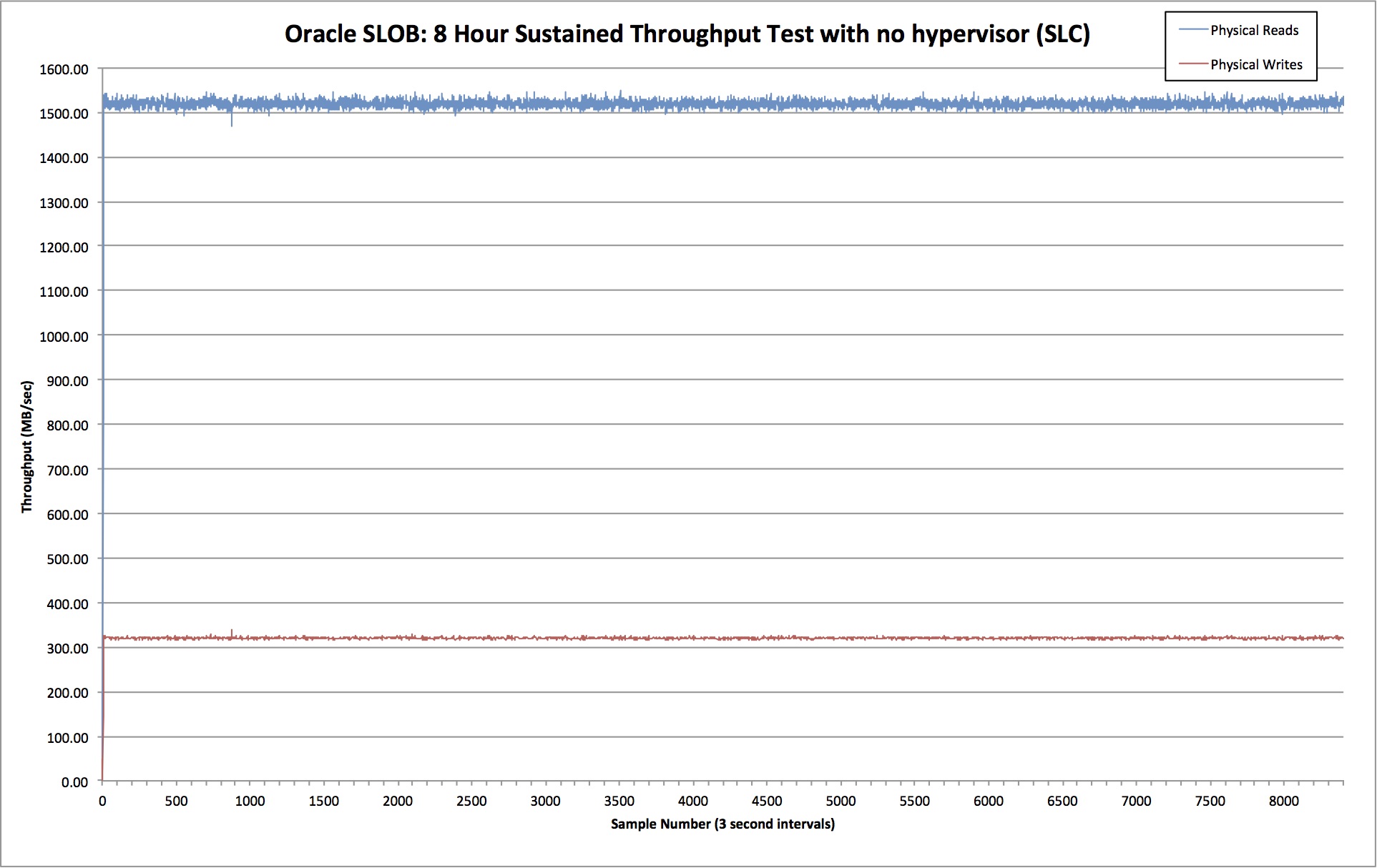
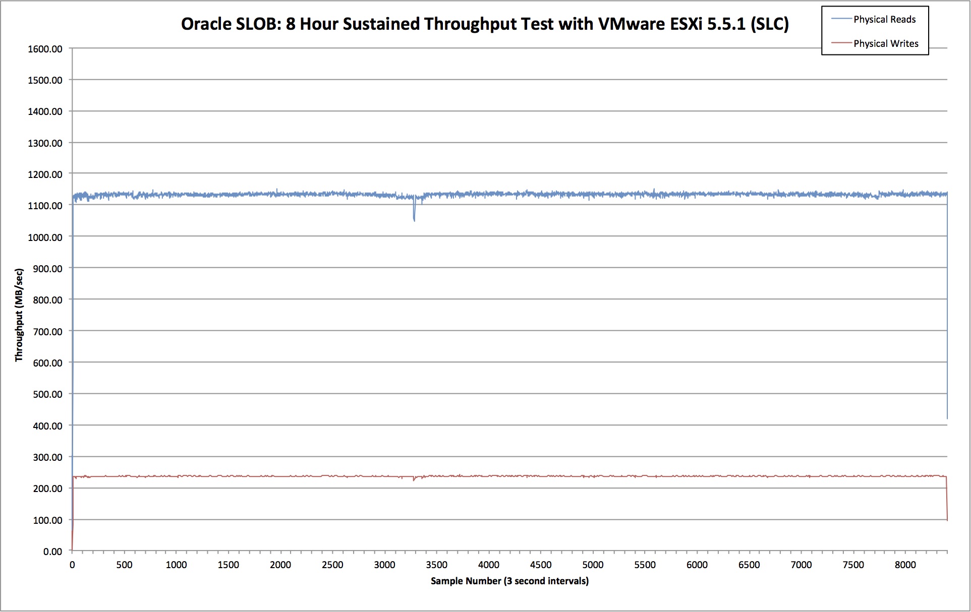
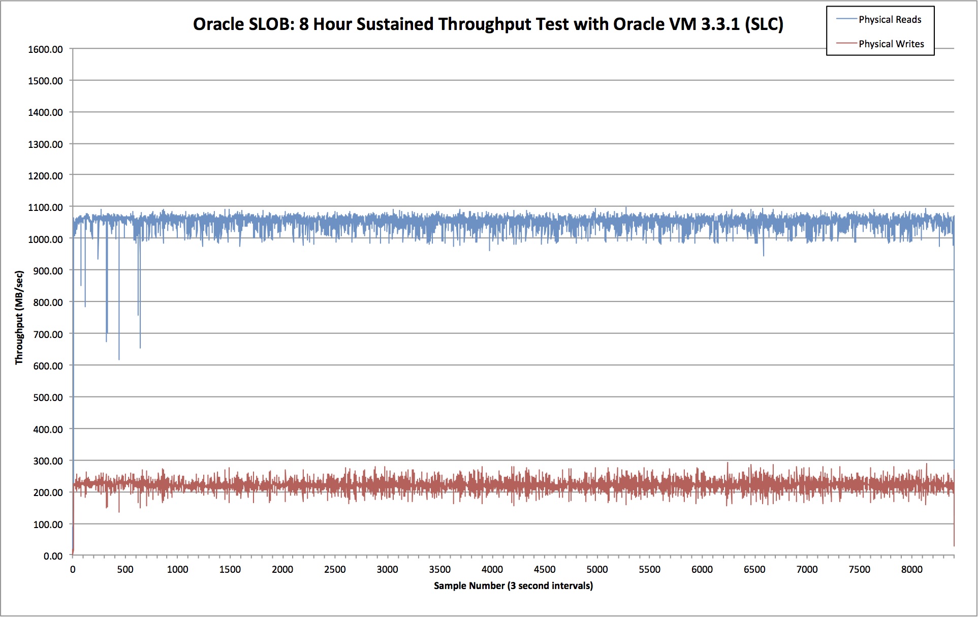


 These are my thoughts and ideas – I’m not claiming them as facts. The data here is not real – it is my attempt at visualising my opinions based on experience and interaction with customers. I’m quite happy to argue my points and concede them in the face of contrary evidence. Of course I’d prefer to substantiate them with proof, but until I (or someone else) can devise a way of doing that, this is all I have. Feel free to add your voice one way or the other… and yes, I am aware that I suck at graphics.


 In
In 

 One thing you do not want to happen when you virtualise your databases onto a consolidated physical platform is to find the ceiling of your I/O capabilities. Every storage system has an upper limit of the number of I/O operations that it can perform per second (known as IOPS) and when that ceiling is reached (known as saturation) things can get painful.
 Forget Big Data. Stop talking about Analytics. There is a trend taking place in the marketplace right now, one that is really happening rather than just being spoken about.


 Finally we come to CPU utilisation. It seems obvious that if you take all of your database environments and consolidate them onto one platform you will need a lot of CPU power to ensure they all coexist peacefully. This is where you really want to be able to overcommit, because CPUs are expensive. Maybe not as hardware components (although they certainly aren’t cheap), but as the major contributor to license cost. Oracle licenses most of its database software by the core, with a “multiplication factor” applied


