One of the results of my employment history is that I tend to take particular interest in the goings on at a certain enterprise software (and hardware!) company based in Redwood Shores. I love watching Oracle’s announcements, press releases, product releases and financial statements to see what they are up to – and I am never more intrigued than when they release a new version of one of their Engineered Systems.
In part this is because I used to work with Exadata a lot and still know many people who do. But the main reason I like Engineered Systems releases is because I believe there is no better indicator of Oracle’s future strategy. Sifting through the deluge of marketing clod, product collateral, datasheets and press releases is like reading the tea leaves – and I’ve been doing it for a long time.
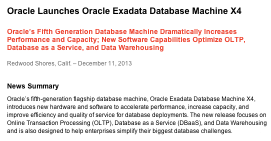
A few weeks ago Oracle released the new “fifth-generation” Exadata Database Machine X4-2, along with the usual avalanche of marketing. Over the last couple of weeks I’ve been throwing it all up in the air to see what lands. Part one of this post will look at the changes, while part two will look at the underlying message.
Database as a Service
The first thing to notice about Exadata X4 is that Oracle Marketing has fallen in love with a new term: database as a service. Previous versions of Exadata were described as being suitable for database consolidation, but in the X4 launch this phrase has been superseded:
Personally I see little difference between consolidation and DBaaS, but I assume the latter has more connotations of cloud computing and so is more fitting for a company attempting to build its own cloud empire. The idea is presumably that you buy Exadata for use in private clouds and use Oracle Cloud for your public cloud service. That’s all very well, but what I find somewhat surprising is the claim that X4 is optimized for OLTP, data warehousing and database-as-a-service. Surely those three workloads encompass everything? Claiming that you have built a solution which is optimized for everything is … shall we say bold?
More Processor Cores = More Licenses
As with previous releases, Oracle has frozen the price of both the Exadata hardware and the Exadata Storage Software licenses (see price lists). This seems like a great result for customers given that the X4 contains significantly faster hardware (see comments section). For example, the Exadata compute nodes change from having 8-core Sandy Bridge versions of the Intel Xeon processor to 12-core Ivy Bridge models. What never ceases to amaze me is the number of people who do not immediately see the consequence of this change: 50% more cores means 50% more database software licenses are required to run the equivalent X4 machine. So while the Exadata storage license cost remains unchanged, the cost of running Oracle Database Enterprise Edition increases by 50%, as does the cost of options such as Oracle RAC, Partitioning, Advanced Compression, the Diagnostic and Tuning Packs, etc etc. And it just so happens that the bits which increase by 50% happen to form the majority of the cost (and don’t forget that the 22% annual fee for support and maintenance will also be going up for them):

So far so boring. Nobody expected something for nothing, despite some of the altruistic statements made to the press. But there’s something much more interesting going on if you look at the X4’s use of flash memory…
Ever-Increasing Capacity
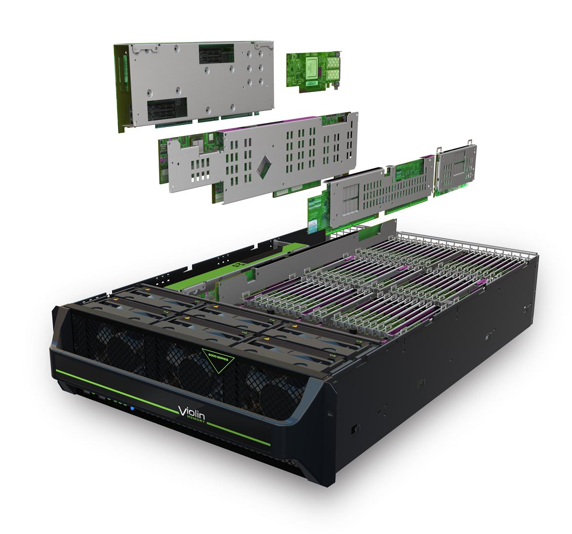
The new Exadata X4 model now contains 44.8TB of raw flash in the form of rebranded LSI Nytro PCIe cards placed in the storage cells. The term “raw“, as always in the storage industry, is used to denote the total amount of flash available prior to any overhead such as RAID, formatting, areas kept aside for garbage collection, etc. Once all of these overheads are added, you end up with a new figure known as “usable” – and it is this amount which describes the area where you can store data.
But hold on, what’s this new term “logical flash capacity” in the press release promising “88 TB per full rack”?
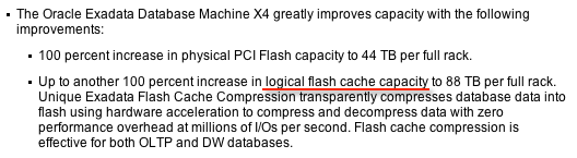
That’s twice the raw capacity! This is an incredible statement, because this so-called “logical” capacity is in fact a complete guess based on compression ratios – which are entirely dependant on your data. And it gets worse when you read the datasheet, which makes the following claim: an “effective flash capacity” of “Up to 448TB“! This is now ten times the raw capacity!
But what is an “effective flash capacity”? Let’s read the small print of the datasheet to find out… Apparently this is the size of the data files that can often be stored in Exadata and be accessed at the speed of flash memory. No guarantees then, you just might get that, if you’re lucky. I thought datasheets where supposed to be about facts?
I am very uncomfortable about this sort of claim, partly because it carries no guarantees, but mainly because it often confuses customers. It’s not inconceivable that a potential customer will mistakenly think they are buying more raw flash capacity than they are actually are. You think not? Then take a look at slide 21 of this Oracle presentation and consider the use of the word “raw”:

Maybe someone can explain to me how that statement can possibly be valid, because to me it looks utterly bewildering.
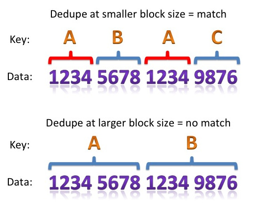
Exadata Smart Flash Cache Compression
The Exadata Smart Flash Cache has been a stalwart of the Exadata machine for many generations, so it is no surprise to see its feature set continually expanding. For the Exadata X4 release, the big feature appears to be Exadata Smart Flash Cache Compression (read more about it here), which allows Oracle to transparently compress data and store it on the PCIe flash cards. It is this feature which Oracle is describing when it claims a “logical flash cache capacity” of 88TB in the press release and the datasheet. Yet according to slide 22 of this Oracle presentation it is a feature which requires the Advanced Compression Option:

As you can see, the author of this slide deck makes the rather brave assumption that most Exadata customers already have licenses for Advanced Compression (something I strongly contest). But either way, does it not seem reasonable that the press release and/or the datasheet should include this statement if they are going to promise such enlarged flash capacities? I’ve looked and looked, but I cannot see this mentioned – even in the infamous small print.
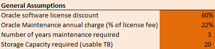
The thing is, right now on the Oracle Store, the Advanced Compression Option is retailing at $11,500 per core. Given that the new Exadata X4 machine now has 192 cores in a full rack (and taking into account the core multiplication factor of 0.5 for Intel Xeon), I calculate the list price of this option as being over $1.1m. Personally, I think that’s a large enough add-on that it ought to be mentioned up front.
Conclusion
As always with Oracle’s Exadata products, there is much to read between the lines. In the second part of this article I’ll be drawing my own conclusions about what the X4 means… stay tuned.


 Storage for DBAs: The strange thing about enterprise databases is that the people who design, manage and support them are often disassociated from the people who pay the bills. In fact, that’s not unusual in enterprise IT, particularly in larger organisations where purchasing departments are often at opposite ends of the org chart to operations and engineering staff.


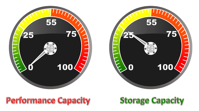
 There are two points I want to make here. One is that the cost of storage is often relatively small in terms of the total cost. If a large amount of money is being spent on licensing the environment it makes sense to ensure that the storage enables better performance, i.e. results in a better return on investment.