Storage for DBAs: Here’s a question I get asked a lot: “Does my database need flash?”. In fact it’s the most common question customers have, followed by the alternative version, “Does my database need SSD?”. In fact, often customers already have some SSDs in their disk arrays but still see poor performance, so really I ought to wind it back a level and call this article, “Does my database need low latency storage?”. This would in fact be a much better headline from a technical perspective, but until I change the name of this site to LowLatencyDBA I’m sticking with the current title.
Flash is no longer a cutting edge new technology, it’s a mainstream product sold by almost every storage vendor. This means that you or your organisation will probably already have some flash sales person beating down your door to flog you some sort of flash product, whether it’s an all-flash array, a hybrid flash/disk system or a set of PCIe flash cards. While these products are diverse in nature, they all share two main characteristics: low latency and large numbers of IOPS. But how do you know whether you really need them?
In a later post I’ll be running through the questions which I think need to be asked in order to whittle down the massive list of flash vendors to the select few capable of servicing your needs. This, of course, will be difficult to achieve without being biased towards my own employer – but that’s a problem for another day. For now, here’s the first (and potentially most important) step: working out whether you actually need low latency flash storage in the first place.
Who Needs Flash?
For the world of databases, there are three main reasons why you might want to switch to low latency flash:
 Acceleration – perhaps the most obvious reason is to go faster. There are many reasons why people desire better performance, but they generally boil down to one of two scenarios: Not Good Enough Now and Not Good Enough For The Future. In the former, bad performance is holding back an application, denying potential revenue or incurring penalties in some way (either SLA-based financial penalties or simply the loss of customers due to poor service levels). In the latter, existing infrastructure is incapable of allowing increased agility, i.e. the ability to do more (offering new services for example, or adding more concurrent users).
Consolidation – always on the mind of CIOs and CTOs is the benefit of consolidating database and server estates. Consolidation brings agility and risk benefits as well as the new and important benefit of cost savings. By consolidating (and standardising) multiple databases onto a smaller pool of servers, organisations save money on hardware, on maintenance and administration, and on the holy grail of all cost savings: software license fees. If you think that sounds like an exaggeration, take a look at this article on Wikibon which demonstrates that Oracle license costs account for 82% of the total cost of a traditional database deployment. Consolidation allows for reduced CPU cores, which means a reduction in the number of licenses, but it also increases I/O as workloads are “stacked” on the same infrastructure. The Wikibon article argues that by moving to flash storage and consolidating, the total cost drops significantly – by around 26% in fact.
Virtualisation – an increasingly prevalent option in the database world. The use of server virtualisation technologies is allowing organisations to move to cloud architectures, where environments are automatically provisioned, managed and migrated across hardware. Virtualisation brings massive agility benefits but also carries a risk because, just like with consolidation, I/O workloads accumulate on the same infrastructure. Unlike consolidation though, virtualisation adds an extra layer of latency, making the I/O even more of a potential bottleneck. Flash systems now make this option practical, as hypervisor vendors begin to realise the potential of flash memory.
There is actually a fourth reason, which is Infrastructure Optimisation. If you have data centres stuffed with disk arrays there is every chance that they can be replaced by a small number of flash arrays, thus reducing power, cooling and real estate requirements and saving large amounts of money. But as this article is primarily targeted at databases I thought I’d leave that one out for now. Consider it the icing on the cake… but don’t forget it, because sometimes it turns out that there’s a lot of icing.
So now we know the reasons why, let’s have a look at which sorts of systems are suitable for flash and which aren’t, starting with the Performance requirement…
Databases Love Flash If…
 They create lots of I/O! I know, it sounds obvious, but more than once I’ve seen customers with CPU-bound applications that generate hardly any I/O. Flash is a fantastic technology, but its not magic.
- There is lots of random I/O. Now don’t take that the wrong way – sequential I/O is good too. But if you currently have a random I/O workload running on a disk system you will see the most dramatic benefit after switching that to flash. Here’s why.
- High amounts of parallelism. The simple fact is that a single process cannot drive anywhere near the amount of I/O that a good flash system can support. If you think of flash as being like a highway, not only is it fast, it’s also wide. Use all the lanes.
- Large IOWAIT times. If you are using an operating system that has a concept of IOWAIT (Linux and most versions of UNIX do, Windows doesn’t) then this can be a great indicator that processes are stuck waiting on I/O. It’s not perfect though, because IOWAIT is actually an idle wait (within the operating system, this is nothing to do with Oracle wait events) so if the system is really busy it may not be present.

Those are all great indicators, but the next two should be considered the golden rules:
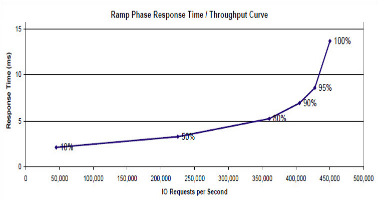
- I/O wait times are high. Essentially we are looking for high latency from the existing storage system. Flash memory systems should deliver I/O with sub-millisecond latency, so if you see an average latency of 8ms on random reads (db file sequential read), for example, you know there is potential for reducing latency to an eighth of its previous average value.
- I/O forms a significant percentage of Database Time. If I/O is only responsible for 5% of database time, no amount of lightening-fast flash is going to give you a big performance boost… your problems are elsewhere. On the other hand, if I/O is comprising a large portion of database time, you have lots of room for improvement. (I plan to post a guide to reading AWR Reports pretty soon)
If any of this is ticking boxes for you, it’s time to consider what flash could do for the performance of your database. On the other hand…
Performance Won’t Improve If…
 There isn’t any I/O. Any flash vendor in the industry would be happy to sell you their products in this situation – and let’s face it you’ll get great latency! – but be realistic. If you don’t generate I/O, what’s the point? Unless of course you aren’t after performance. If consolidation, virtualisation or infrastructure optimisation is your aim, there could be a benefit. Also, consider the size of your memory components – if your database produces no physical I/O, could you consider reducing the size of the buffer cache? One of the big benefits of flash to consolidation is the ability to reduce SGA sizes and thus fit more databases onto the same DRAM-restricted server.
- Single threaded workloads. Sure your application will run slightly faster, but will that speed-up be enough to justify the change of infrastructure? I’m not ruling this out – I have customers with single-threaded ETL jobs that bought flash because it was easier (and cheaper) than rewriting legacy code, but the impact of low-latency storage may well be reduced.
- Application serialisation points. A session waiting on a lock will not wait any faster! Basically, if your application regularly ties itself in a knot with locks and contention issues, putting it on flash may well just increase the speed at which you hit those problems. Sometimes people use flash to overcome bad programming, but it’s by no means guaranteed to work.
- CPU-bound systems. CPU starvation is a CPU problem, not an I/O problem. If anything, moving to low-latency storage will reduce the amount of time CPUs spent waiting on I/O and thus increase the amount of time they spend working, i.e. in a busy state. If your CPU is close to the limit and you remove the ballast that is a disk system, you might find that you hit the limit very quickly.

If you are unfortunate enough to be struggling with a badly-performing application that fits into one of these areas, flash probably isn’t the magic bullet you’re looking for.
Consolidation and Virtualisation
This is a different area where it’s no longer valid to only look at individual databases and their workloads. The key factor for both of these areas is density i.e. the number of databases or virtual machines that can fit on a single physical server. The main challenges here are memory usage and I/O generation: databases SGAs tend to be large, but flash allows for the possibility of reducing the buffer cache; while I/O generation is a problem in the disk world because consolidated workloads tend to create more random I/O. Of course, with flash that’s not really a problem. I’ve written a number of articles on consolidation and virtualisation in the past – I’m sure I’ll be writing more about them in the future too.
Summary
I work for a flash vendor – we want you to buy our products. We have competitors who want you to buy their products instead. If everyone in the industry is telling you to buy flash, how do you know if it’s relevant to you? Here’s my advice: make them speak your language and then check their claims against what you can see yourself.
Take some time to understand your workload. Look at the amount of I/O generated and the latency experienced; look at how random the workload is and the ratio of reads to writes (I’ll post a guide for this soon). Ask your (potential) flash vendor how much benefit you will see from your existing storage and then get them to explain why. If you’re a database person, make them speak in your language – don’t accept someone talking in the language of storage. Likewise if you’re an application person make them explain the benefits from an application perspective. You’re the customer, after all.
If your flash vendor can’t communicate with you in your language to explain the benefit you will see, there’s only one course of action: Get rid of them in a flash.
Footnote
Incidentally, if you live outside the UK and you’re wondering about the picture at the top of this article, check out this. If you live inside the UK you will know it’s a Cillit Bang reference… unless you live in a cave and shun the outside world – in which case, how are you reading this?